Global Bullies, Climate Models and Dishonesty in Climate Science

By Dr. DAVID EVANS | THE REAL AGENDA | MAY 25, 2012

The debate about global warming has reached ridiculous proportions and is full of micro thin half-truths and misunderstandings. I am a scientist who was on the carbon gravy train, understands the evidence,  was once an alarmist, but am now a skeptic. Watching this issue unfold has been amusing but, lately, worrying. This issue is tearing society apart, making fools and liars out of our politicians.

Let’s set a few things straight.

The whole idea that carbon dioxide is the main cause of the recent global warming is based on a guess that was proved false by empirical evidence during the 1990s. But the gravy train was too big, with too many jobs, industries, trading profits, political careers, and the possibility of world government and total control riding on the outcome. So rather than admit they were wrong, the governments, and their tame climate scientists, now cheat and lie outrageously to maintain the fiction that carbon dioxide is a dangerous pollutant.

Let’s be perfectly clear. Carbon dioxide is a greenhouse gas, and other things being equal, the more carbon dioxide in the air, the warmer the planet. Every bit of carbon dioxide that we emit warms the planet. But the issue is not whether carbon dioxide warms the planet, but how much.

Most scientists, on both sides, also agree on how much a given increase in the level of carbon dioxide raises the planet’s temperature, if just the extra carbon dioxide is considered. These calculations come from laboratory experiments; the basic physics have been well known for a century.

The disagreement comes about what happens next.

The planet reacts to that extra carbon dioxide, which changes everything. Most critically, the extra warmth causes more water to evaporate from the oceans. But does the water hang around and increase the height of moist air in the atmosphere, or does it simply create more clouds and rain? Back in 1980, when the carbon dioxide theory started, no one knew. The alarmists guessed that it would increase the height of moist air around the planet, which would warm the planet even further, because the moist air is also a greenhouse gas.

This is the core idea of every official climate model: for each bit of warming due to carbon dioxide, they claim it ends up causing three bits of warming due to the extra moist air. The climate models amplify the carbon dioxide warming by a factor of three – so two thirds of their projected warming is due to extra moist air (and other factors), only one third is due to extra carbon dioxide.

I’ll bet you didn’t know that. Hardly anyone in the public does, but it’s the core of the issue. All the disagreements, lies, and misunderstanding spring from this. The alarmist case is based on this guess about moisture in the atmosphere, and there is simply no evidence for the amplification that is at the core of their alarmism. Which is why the alarmists keep so quiet about it and you’ve never heard of it before. And it tells you what a poor job the media have done in covering this issue.

Weather balloons had been measuring the atmosphere since the 1960s, many thousands of them every year. The climate models all predict that as the planet warms, a hot-spot of moist air will develop over the tropics about 10km up, as the layer of moist air expands upwards into the cool dry air above. During the warming of the late 1970s, 80s, and 90s, the weather balloons found no hot-spot. None at all. Not even a small one. This evidence proves that the climate models are fundamentally flawed, that they greatly overestimate the temperature increases due to carbon dioxide.

This evidence first became clear around the mid 1990s.

At this point official “climate science” stopped being a science. You see, in science empirical evidence always trumps theory, no matter how much you are in love with the theory. If theory and evidence disagree, real scientists scrap the theory. But official climate science ignored the crucial weather balloon evidence, and other subsequent evidence that backs it up, and instead clung to their carbon dioxide theory — that just happens to keep them in well-paying jobs with lavish research grants, and gives great political power to their government masters.

There are now several independent pieces of evidence showing that the earth responds to the warming due to extra carbon dioxide by dampening the warming. Every long-lived natural system behaves this way, counteracting any disturbance, otherwise the system would be unstable. The climate system is no exception, and now we can prove it.

But the alarmists say the exact opposite, that the climate system amplifies any warming due to extra carbon dioxide, and is potentially unstable. Surprise surprise, their predictions of planetary temperature made in 1988 to the US Congress, and again in 1990, 1995, and 2001, have all proved much higher than reality.

They keep lowering the temperature increases they expect, from 0.30C per decade in 1990, to 0.20C per decade in 2001, and now 0.15C per decade – yet they have the gall to tell us “it’s worse than expected”. These people are not scientists. They over-estimate the temperature increases due to carbon dioxide, selectively deny evidence, and now they cheat and lie to conceal the truth.

One way they cheat is in the way they measure temperature.

The official thermometers are often located in the warm exhaust of air conditioning outlets, over hot tarmac at airports where they get blasts of hot air from jet engines, at wastewater plants where they get warmth from decomposing sewage, or in hot cities choked with cars and buildings. Global warming is measured in tenths of a degree, so any extra heating nudge is important. In the US, nearly 90% of official thermometers surveyed by volunteers violate official siting requirements that they not be too close to an artificial heating source. Nearly 90%! The photos of these thermometers are on the Internet; you can get to them via the corruption paper at my site, sciencespeak.com. Look at the photos, and you’ll never trust a government climate scientist again.

They place their thermometers in warm localities, and call the results “global” warming. Anyone can understand that this is cheating. They say that 2010 is the warmest recent year, but it was only the warmest at various airports, selected air conditioners, and certain car parks.

Global temperature is also measured by satellites, which measure nearly the whole planet 24/7 without bias. The satellites say the hottest recent year was 1998, and that since 2001 the global temperature has leveled off.

So it’s a question of trust.

If it really is warming up as the government climate scientists say, why do they present only the surface thermometer results and not mention the satellite results? And why do they put their thermometers near artificial heating sources? This is so obviously a scam now.

So what is really going on with the climate?

The earth has been in a warming trend since the depth of the Little Ice Age around 1680. Human emissions of carbon dioxide were negligible before 1850 and have nearly all come after WWII, so human carbon dioxide cannot possibly have caused the trend. Within the trend, the Pacific Decadal Oscillation causes alternating global warming and cooling for 25 – 30 years at a go in each direction. We have just finished a warming phase, so expect mild global cooling for the next two decades.

We are now at an extraordinary juncture.

Official climate science, which is funded and directed entirely by government, promotes a theory that is based on a guess about moist air that is now a known falsehood. Governments gleefully accept their advice, because the only way to curb emissions are to impose taxes and extend government control over all energy use. And to curb emissions on a world scale might even lead to world government — how exciting for the political class!

A carbon tax?

Even if Australia stopped emitting all carbon dioxide tomorrow, completely shut up shop and went back to the stone age, according to the official government climate models it would be cooler in 2050 by about 0.015 degrees. But their models exaggerate tenfold – in fact our sacrifices would make the planet in 2050 a mere 0.0015 degrees cooler!

Sorry, but you’ve been had.

Finally, to those of you who still believe the planet is in danger from our carbon dioxide emissions: sorry, but you’ve been had. Yes carbon dioxide a cause of global warming, but it’s so minor it’s not worth doing much about.

This article first appeared on JoNova

Dr David Evans consulted full-time for the Australian Greenhouse Office (now the Department of Climate Change) from 1999 to 2005, and part-time 2008 to 2010, modeling Australia’s carbon in plants, debris, mulch, soils, and forestry and agricultural products. Evans is a mathematician and engineer, with six university degrees including a PhD from Stanford University in electrical engineering. The area of human endeavor with the most experience and sophistication in dealing with feedbacks and analyzing complex systems is electrical engineering, and the most crucial and disputed aspects of understanding the climate system are the feedbacks. The evidence supporting the idea that CO2 emissions were the main cause of global warming reversed itself from 1998 to 2006, causing Evans to move from being a warmist to a skeptic.

Climate Coup: The Politics

How the regulating class is using bogus claims about climate change to entrench and extend their economic privileges and political control.

By DR. DAVID EVANS | SPPI | APRIL 24, 2012

THE SCIENCE

The sister article Climate Coup—The Science contains the science foundation for this essay. It checks the track record of the climate models against our best and latest data, from impeccable sources. It details how you can download this data yourself. It finds that the climate models got all their major predictions wrong:

The latter two items are especially pertinent, because they show that the crucial amplification by water feedbacks (mainly humidity and clouds),1 assumed by the models, does not exist in reality. Modelers guessed that of the forces on temperature, only CO2 has changed significantly since 1750. The amplification by water feedbacks causes two-thirds of the warming predicted by the models, while carbon dioxide only directly causes one third. The presence of the amplification in the models, but not in reality, explains why the models overestimated recent warming.

WHO ARE YOU GOING TO BELIEVE — THE GOVERNMENT CLIMATE SCIENTISTS OR YOUR OWN LYING EYES?

The climate models are incompatible with the data. You cannot believe both the theory of dangerous manmade global warming and the data, because they cannot both be right.
In science, data trumps theory. If data and theory disagree, as they do here, people of a more scientific bent go with the data and scrap the theory.

But in politics we usually go with authority figures, who in this case are the government climate scientists and the western governments—and they strongly support the theory. Many people simply cannot get past the fact that nearly all the authority figures believe the theory. To these people the data is simply irrelevant. Society needs most people to follow authority most of the time, just like an army needs soldiers who do not question orders.

The world’s climate scientists are almost all employed by western governments. They usually don’t pay you to do climate research unless you say you believe manmade global warming is dangerous, and it has been that way for more than 20 years.2 The result is a near-unanimity that is unusual for a theory in such an immature science.

SIDESHOWS INSTEAD OF THE WHOLE TRUTH

The government climate scientists and mainstream media have kept at least two important truths from the public and the politicians:

1. Two thirds of the warming predicted by the climate models is due to amplification by the water feedbacks, and only one third is directly due to CO2.

2. The dispute among scientists is about the water feedbacks. There is no dispute among serious scientists about the direct effect of CO2.

They seek to persuade with partial truths and omissions, not telling the truth in a disinterested manner. Instead, we are treated to endless sideshows. Issues such as Arctic ice, polar bears, bad weather , or the supposed psychological sickness of those opposing the authorities, tell us nothing about the causes of global warming. They divert public attention and the water feedbacks escapes scrutiny—hidden in plain sight, but never under public discussion.

THE SILENCE OF THE MAINSTREAM MEDIA

The data presented in Climate Coup—The Science is plainly relevant, publicly available, and impeccably sourced from our best instruments—satellites, Argo, and the weather balloons. Yet it never appears in the mainstream media. Have you ever seen it?

If the mainstream media were interested in the truth, they would seek out the best and latest data and check the predictions against the data. They don’t.

The newspapers are happy to devote acres of newsprint to the climate sideshows or to demonizing anyone who criticizes the theory. So why are they unwilling to publish the most relevant data?
Global warning has been a big issue for years. Yet all of the world’s investigative journalists—those cynical, hard-bitten, clever, incorruptible, scandal-sniffing reporters of the vital truths who are celebrated in their own press—all of them just happen not to notice

that the climate models get all their major predictions wrong? Really? Even though we point it out to them?

Good detectives do not overlook clues. The presented data contains half a dozen clues of brick-in-your-face subtlety. How could anyone miss them? Will the journalists who read this paragraph now follow the instructions on downloading the data, and report on what they find? No.

Perhaps they think it’s all too complicated, that it will make our brains hurt? A story with two numbers is too hard? No, we all understand a graph of temperature over time and can spot trends. Judging by the huge response on the Internet, the public want well-explained technical details about the climate.

The government climate scientists and their climate models said it would warm like this and heat up the atmosphere like that. But it didn’t, just download the data and check.

The media are withholding this data, so the “climate debate” is obviously not about science or truth. It must be about politics and power. Reluctantly, uncomfortably, the only possible conclusion is that the media don’t want to investigate the claims of the government climate scientists. Why? Who benefits?

Read Full Article →

The Weather Isn’t Getting Weirder

The latest research belies the idea that storms are getting more extreme.

WSJ

By Anne Jolis

Last week a severe storm froze Dallas under a sheet of ice, just in time to disrupt the plans of the tens of thousands of (American) football fans descending on the city for the Super Bowl. On the other side of the globe, Cyclone Yasi slammed northeastern Australia, destroying homes and crops and displacing hundreds of thousands of people.

No evidence in this study suggests that larger storms, tropical or otherwise are caused by human activity and the emissions that come with it.


Some climate alarmists would have us believe that these storms are yet another baleful consequence of man-made CO2 emissions. In addition to the latest weather events, they also point to recent cyclones in Burma, last winter’s fatal chills in Nepal and Bangladesh, December’s blizzards in Britain, and every other drought, typhoon and unseasonable heat wave around the world.

But is it true? To answer that question, you need to understand whether recent weather trends are extreme by historical standards. The Twentieth Century Reanalysis Project is the latest attempt to find out, using super-computers to generate a dataset of global atmospheric circulation from 1871 to the present.

As it happens, the project’s initial findings, published last month, show no evidence of an intensifying weather trend. “In the climate models, the extremes get more extreme as we move into a doubled CO2 world in 100 years,” atmospheric scientist Gilbert Compo, one of the researchers on the project, tells me from his office at the University of Colorado, Boulder. “So we were surprised that none of the three major indices of climate variability that we used show a trend of increased circulation going back to 1871.”

In other words, researchers have yet to find evidence of more-extreme weather patterns over the period, contrary to what the models predict. “There’s no data-driven answer yet to the question of how human activity has affected extreme weather,” adds Roger Pielke Jr., another University of Colorado climate researcher.

We do know that carbon dioxide and other gases trap and re-radiate heat. We also know that humans have emitted ever-more of these gases since the Industrial Revolution. What we don’t know is exactly how sensitive the climate is to increases in these gases versus other possible factors—solar variability, oceanic currents, Pacific heating and cooling cycles, planets’ gravitational and magnetic oscillations, and so on.

Given the unknowns, it’s possible that even if we spend trillions of dollars, and forgo trillions more in future economic growth, to cut carbon emissions to pre-industrial levels, the climate will continue to change—as it always has.

That’s not to say we’re helpless. There is at least one climate lesson that we can draw from the recent weather: Whatever happens, prosperity and preparedness help. North Texas’s ice storm wreaked havoc and left hundreds of football fans stranded, cold, and angry. But thanks to modern infrastructure, 21st century health care, and stockpiles of magnesium chloride and snow plows, the storm caused no reported deaths and Dallas managed to host the big game on Sunday.

Compare that outcome to the 55 people who reportedly died of pneumonia, respiratory problems and other cold-related illnesses in Bangladesh and Nepal when temperatures dropped to just above freezing last winter. Even rich countries can be caught off guard: Witness the thousands stranded when Heathrow skimped on de-icing supplies and let five inches of snow ground flights for two days before Christmas. Britain’s GDP shrank by 0.5% in the fourth quarter of 2010, for which the Office of National Statistics mostly blames “the bad weather.”

Arguably, global warming was a factor in that case. Or at least the idea of global warming was. The London-based Global Warming Policy Foundation charges that British authorities are so committed to the notion that Britain’s future will be warmer that they have failed to plan for winter storms that have hit the country three years running.

A sliver of the billions that British taxpayers spend on trying to control their climes could have bought them more of the supplies that helped Dallas recover more quickly. And, with a fraction of that sliver of prosperity, more Bangladeshis and Nepalis could have acquired the antibiotics and respirators to survive their cold spell.

A comparison of cyclones Yasi and Nargis tells a similar story: As devastating as Yasi has been, Australia’s infrastructure, medicine, and emergency protocols meant the Category 5 storm has killed only one person so far. Australians are now mulling all the ways they could have better protected their property and economy.

But if they feel like counting their blessings, they need only look to the similar cyclone that hit the Irrawaddy Delta in 2008. Burma’s military regime hadn’t allowed for much of an economy before the cyclone, but Nargis destroyed nearly all the Delta had. Afterwards, the junta blocked foreign aid workers from delivering needed water purification and medical supplies. In the end, the government let Nargis kill more than 130,000 people.

Global-warming alarmists insist that economic activity is the problem, when the available evidence show it to be part of the solution. We may not be able to do anything about the weather, extreme or otherwise. But we can make sure we have the resources to deal with it when it comes.

Climate Sensitivity Reconsidered Part 1

A special report from Christopher Monckton of Brenchley for all Climate Alarmists, Consensus Theorists and Anthropogenic Global Warming Supporters

January 20, 2011

Abstract

The Intergovernmental Panel on Climate Change (IPCC, 2007) concluded that anthropogenic CO2 emissions probably
caused more than half of the “global warming” of the past 50 years and would cause further rapid warming. However,
global mean surface temperature TS has not risen since 1998 and may have fallen since late 2001. The present analysis
suggests that the failure of the IPCC’s models to predict this and many other climatic phenomena arises from defects in its
evaluation of the three factors whose product is climate sensitivity:

1) Radiative forcing ΔF;
2) The no-feedbacks climate sensitivity parameter κ; and
3) The feedback multiplier f.
Some reasons why the IPCC’s estimates may be excessive and unsafe are explained. More importantly, the conclusion is
that, perhaps, there is no “climate crisis”, and that currently-fashionable efforts by governments to reduce anthropogenic
CO2 emissions are pointless, may be ill-conceived, and could even be harmful.

The context

LOBALLY-AVERAGED land and sea surface absolute temperature TS has not risen since 1998 (Hadley Center; US National Climatic Data Center; University of Alabama at Huntsville; etc.). For almost seven years, TS may even have fallen (Figure 1). There may be no new peak until 2015 (Keenlyside et al., 2008).

The models heavily relied upon by the Intergovernmental Panel on Climate Change (IPCC) had not projected this multidecadal stasis in “global warming”; nor (until trained ex post facto) the fall in TS from 1940-1975; nor 50 years’ cooling in Antarctica (Doran et al., 2002) and the Arctic (Soon, 2005); nor the absence of ocean warming since 2003 (Lyman et al., 2006; Gouretski & Koltermann, 2007); nor the onset, duration, or intensity of the Madden-Julian intraseasonal oscillation, the Quasi-Biennial Oscillation in the tropical stratosphere, El Nino/La Nina oscillations, the Atlantic Multidecadal Oscillation, or the Pacific Decadal Oscillation that has recently transited from its warming to its cooling phase (oceanic oscillations which, on their own, may account for all of the observed warmings and coolings over the past half-century: Tsonis et al., 2007); nor the magnitude nor duration of multicentury events such as the Medieval Warm Period or the Little Ice Age; nor the cessation since 2000 of the previously-observed growth in atmospheric methane concentration (IPCC, 2007); nor the active 2004 hurricane season; nor the inactive subsequent seasons; nor the UK flooding of 2007 (the Met Office had forecast a summer of prolonged droughts only six weeks previously); nor the solar Grand Maximum of the past 70 years, during which the Sun was more active, for longer, than at almost any
similar period in the past 11,400 years (Hathaway, 2004; Solanki et al., 2005); nor the consequent surface “global warming” on Mars, Jupiter, Neptune’s largest moon, and even distant Pluto; nor the eerily- continuing 2006 solar minimum; nor the consequent, precipitate decline of ~0.8 °C in TS from January 2007 to May 2008 that has canceled out almost all of the observed warming of the 20th century.

Figure 1
Mean global surface temperature anomalies (°C), 2001-2008


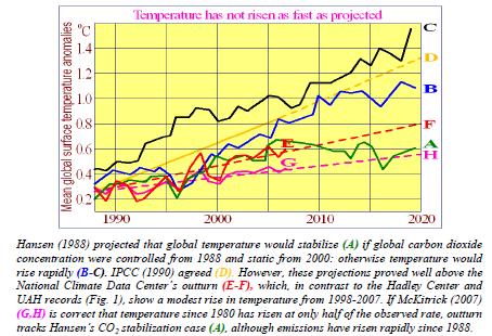
An early projection of the trend in TS in response to “global warming” was that of Hansen (1988), amplifying Hansen (1984) on quantification of climate sensitivity. In 1988, Hansen showed Congress a graph projecting rapid increases in TS to 2020 through “global warming” (Fig. 2):

Figure 2
Global temperature projections and outturns, 1988-2020


To what extent, then, has humankind warmed the world, and how much warmer will the world become if the current rate of increase in anthropogenic CO2 emissions continues? Estimating “climate sensitivity” – the magnitude of the change in TS after doubling CO2 concentration from the pre-industrial 278 parts per million to ~550 ppm – is the central question in the scientific debate about the climate. The official answer is given in IPCC (2007):

“It is very likely that anthropogenic greenhouse gas increases caused most of the observed increase in [TS] since the mid-20th century. … The equilibrium global average warming expected if carbon dioxide concentrations were to be sustained at 550 ppm is likely to be in the range 2-4.5 °C above pre-industrial values, with a best estimate of about 3 °C.”

Here as elsewhere the IPCC assigns a 90% confidence interval to “very likely”, rather than the customary 95% (two standard deviations). There is no good statistical basis for any such quantification, for the object to which it is applied is, in the formal sense, chaotic. The climate is “a complex, nonlinear, chaotic object” that defies long-run prediction of its future states (IPCC, 2001), unless the initial state of its millions of variables is known to a precision that is in practice unattainable, as Lorenz (1963; and see Giorgi, 2005) concluded in the celebrated paper that founded chaos theory –
“Prediction of the sufficiently distant future is impossible by any method, unless the present conditions are known exactly. In view of the inevitable inaccuracy and incompleteness of weather observations, precise, very-long-range weather forecasting would seem to be nonexistent.”  The Summary for Policymakers in IPCC (2007) says –“The CO2 radiative forcing increased by 20% in the last 10 years (1995-2005).”

Natural or anthropogenic CO2 in the atmosphere induces a “radiative forcing” ΔF, defined by IPCC (2001: ch.6.1) as a change in net (down minus up) radiant-energy flux at the tropopause in response to a perturbation. Aggregate forcing is natural (pre-1750) plus anthropogenic-era (post-1750) forcing. At 1990, aggregate forcing from CO2 concentration was ~27 W m–2 (Kiehl & Trenberth, 1997). From 1995-2005, CO2 concentration rose 5%, from 360 to 378 W m–2, with a consequent increase in aggregate forcing (from Eqn. 3 below) of ~0.26 W m–2, or <1%. That is one-twentieth of the value
stated by the IPCC. The absence of any definition of “radiative forcing” in the 2007 Summary led many to believe that the aggregate (as opposed to anthropogenic) effect of CO2 on TS had increased by 20% in 10 years. The IPCC – despite requests for correction – retained this confusing statement in its report.  Such solecisms throughout the IPCC’s assessment reports (including the insertion, after the scientists had completed their final draft, of a table in which four decimal points had been right-shifted so as to multiply tenfold the observed contribution of ice-sheets and glaciers to sea-level rise), combined with a heavy reliance upon computer models unskilled even in short-term projection, with initial values of key
variables unmeasurable and unknown, with advancement of multiple, untestable, non-Popperfalsifiable theories, with a quantitative assignment of unduly high statistical confidence levels to nonquantitative statements that are ineluctably subject to very large uncertainties, and, above all, with the now-prolonged failure of TS to rise as predicted (Figures 1, 2), raise questions about the reliability and hence policy-relevance of the IPCC’s central projections.

Dr. Rajendra Pachauri, chairman of the UN Intergovernmental Panel on Climate Change (IPCC), has recently said that the IPCC’s evaluation of climate sensitivity must now be revisited. This paper is a respectful contribution to that re-examination.

The IPCC’s method of evaluating climate sensitivity

We begin with an outline of the IPCC’s method of evaluating climate sensitivity. For clarity we will concentrate on central estimates. The IPCC defines climate sensitivity as equilibrium temperature change ΔTλ in response to all anthropogenic-era radiative forcings and consequent “temperature feedbacks” – further changes in TS that occur because TS has already changed in response to a forcing – arising in response to the doubling of pre-industrial CO2 concentration (expected later this century).  ΔTλ is, at its simplest, the product of three factors: the sum ΔF2x of all anthropogenic-era radiative forcings at CO2 doubling; the base or “no-feedbacks” climate sensitivity parameter κ; and the feedback
multiplier f, such that the final or “with-feedbacks” climate sensitivity parameter λ = κ f. Thus –

ΔTλ = ΔF2x κ f = ΔF2x λ, (1)
where f = (1 – bκ)–1, (2)

such that b is the sum of all climate-relevant temperature feedbacks. The definition of f in Eqn. (2) will be explained later. We now describe seriatim each of the three factors in ΔTλ: namely, ΔF2x, κ, and f.

1. Radiative forcing ΔFCO2, where (C/C0) is a proportionate increase in CO2 concentration, is given by several formulae in IPCC (2001, 2007). The simplest, following Myrhe (1998), is Eqn. (3) –

ΔFCO2 ≈ 5.35 ln(C/C0) ==> ΔF2xCO2 ≈ 5.35 ln 2 ≈ 3.708 W m–2. (3)

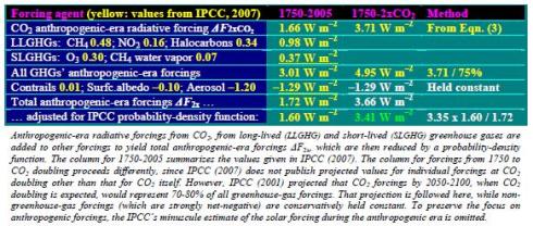
To ΔF2xCO2 is added the slightly net-negative sum of all other anthropogenic-era radiative forcings, calculated from IPCC values (Table 1), to obtain total anthropogenic-era radiative forcing ΔF2x at CO2 doubling (Eqn. 3). Note that forcings occurring in the anthropogenic era may not be anthropogenic.

Table 1
Evaluation of ΔF2x from the IPCC’s anthropogenic-era forcings


From the anthropogenic-era forcings summarized in Table 1, we obtain the first of the three factors –
ΔF2x ≈ 3.405 Wm–2. (4)

Continue to Part 2

Climate Sensitivity Reconsidered Part 2

A special report from Christopher Monckton of Brenchley to all Climate Alarmists, Consensus Theorists and Anthropogenic Global Warming Supporters

Continues from Part 1

2. The base or “no-feedbacks” climate sensitivity parameter κ, where ΔTκ is the response of TS to radiative forcings ignoring temperature feedbacks, ΔTλ is the response of TS to feedbacks as well as forcings, and b is the sum in W m–2 °K–1 of all individual temperature feedbacks, is –

κ = ΔTκ / ΔF2x °K W–1 m2, by definition; (5)
= ΔTλ / (ΔF2x + bΔTλ) °K W–1 m2. (6)

In Eqn. (5), ΔTκ, estimated by Hansen (1984) and IPCC (2007) as 1.2-1.3 °K at CO2 doubling, is the change in surface temperature in response to a tropopausal forcing ΔF2x, ignoring any feedbacks.  ΔTκ is not directly mensurable in the atmosphere because feedbacks as well as forcings are present.  Instruments cannot distinguish between them. However, from Eqn. (2) we may substitute 1 / (1 – bκ) for f in Eqn. (1), rearranging terms to yield a useful second identity, Eqn. (6), expressing κ in terms of ΔTλ, which is mensurable, albeit with difficulty and subject to great uncertainty (McKitrick, 2007).  IPCC (2007) does not mention κ and, therefore, provides neither error-bars nor a “Level of Scientific
Understanding” (the IPCC’s subjective measure of the extent to which enough is known about a variable to render it useful in quantifying climate sensitivity). However, its implicit value κ ≈ 0.313 °K W–1 m2, shown in Eqn. 7, may be derived using Eqns. 9-10 below, showing it to be the reciprocal of the estimated “uniform-temperature” radiative cooling response–

“Under these simplifying assumptions the amplification [f] of the global warming from a feedback parameter [b] (in W m–2 °C–1) with no other feedbacks operating is 1 / (1 –[bκ –1]), where [–κ –1] is the ‘uniform temperature’ radiative cooling response (of value approximately –3.2 W m–2 °C–1; Bony et al., 2006). If n independent feedbacks operate, [b] is replaced by (λ1 + λ 2+ … λ n).” (IPCC, 2007: ch.8, footnote).

Thus, κ ≈ 3.2–1 ≈ 0.313 °K W–1 m2. (7)

3. The feedback multiplier f is a unitless variable by which the base forcing is multiplied to take account of mutually-amplified temperature feedbacks. A “temperature feedback” is a change in TS that occurs precisely because TS has already changed in response to a forcing or combination of forcings.  An instance: as the atmosphere warms in response to a forcing, the carrying capacity of the space occupied by the atmosphere for water vapor increases near-exponentially in accordance with the Clausius-Clapeyron relation. Since water vapor is the most important greenhouse gas, the growth in its
concentration caused by atmospheric warming exerts an additional forcing, causing temperature to rise further. This is the “water-vapor feedback”. Some 20 temperature feedbacks have been described, though none can be directly measured. Most have little impact on temperature. The value of each feedback, the interactions between feedbacks and forcings, and the interactions between feedbacks and other feedbacks, are subject to very large uncertainties.

Each feedback, having been triggered by a change in atmospheric temperature, itself causes a temperature change. Consequently, temperature feedbacks amplify one another. IPCC (2007: ch.8) defines f in terms of a form of the feedback-amplification function for electronic circuits given in Bode (1945), where b is the sum of all individual feedbacks before they are mutually amplified:

f = (1 – bκ)–1 (8)
= ΔTλ / ΔTκ

Note the dependence of f not only upon the feedback-sum b but also upon κ –

ΔTλ = (ΔF + bΔTλ)κ
==> ΔTλ (1 – bκ) = ΔFκ
==> ΔTλ = ΔFκ(1 – bκ)–1
==> ΔTλ / ΔF = λ = κ(1 – bκ)–1 = κf
==> f = (1 – bκ)–1 ≈ (1 – b / 3.2)–1
==> κ ≈ 3.2–1 ≈ 0.313 °K W–1 m2. (9)

Equivalently, expressing the feedback loop as the sum of an infinite series,

ΔTλ = ΔFκ + ΔFκ 2b + ΔFκ 2b2 + …
= ΔFκ(1 + κb + κb2 + …)
= ΔFκ(1 – κb)–1
= ΔFκf
==> λ = ΔTλ /ΔF = κf (10)

Figure 3
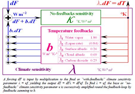
Bode (1945) feedback amplification schematic


For the first time, IPCC (2007) quantifies the key individual temperature feedbacks summing to b:
“In AOGCMs, the water vapor feedback constitutes by far the strongest feedback, with a multi-model mean and standard deviation … of 1.80 ± 0.18 W m–2 K–1, followed by the negative lapse rate feedback (–0.84 ± 0.26 W m–2 K–1) and the surface albedo feedback (0.26 ± 0.08 W m–2 K–1). The cloud feedback mean is 0.69 W m–2 K–1 with a very large inter-model spread of ±0.38 W m–2K–1.” (Soden & Held, 2006).

To these we add the CO2 feedback, which IPCC (2007, ch.7) separately expresses not as W m–2 °K–1 but as concentration increase per CO2 doubling: [25, 225] ppmv, central estimate q = 87 ppmv. Where p is concentration at first doubling, the proportionate increase in atmospheric CO2 concentration from the CO2 feedback is o = (p + q) / p = (556 + 87) / 556 ≈ 1.16. Then the CO2 feedback is –λCO2 = z ln(o) / dTλ ≈ 5.35 ln(1.16) / 3.2 ≈ 0.25 Wm–2 K–1. (11) The CO2 feedback is added to the previously-itemized feedbacks to complete the feedback-sum b:

b = 1.8 – 0.84 + 0.26 + 0.69 + 0.25 ≈ 2.16 Wm–2 ºK–1, (12)

so that, where κ = 0.313, the IPCC’s unstated central estimate of the value of the feedback factor f is at the lower end of the range f = 3-4 suggested in Hansen et al. (1984) –

f = (1 – bκ)–1 ≈ (1 – 2.16 x 0.313)–1 ≈ 3.077. (13)

Final climate sensitivity ΔTλ, after taking account of temperature feedbacks as well as the forcings that triggered them, is simply the product of the three factors described in Eqn. (1), each of which we have briefly described above. Thus, at CO2 doubling, –

ΔTλ = ΔF2x κ f ≈ 3.405 x 0.313 x 3.077 ≈ 3.28 °K (14)

IPCC (2007) gives dTλ on [2.0, 4.5] ºK at CO2 doubling, central estimate dTλ ≈ 3.26 °K, demonstrating that the IPCC’s method has been faithfully replicated. There is a further checksum, –

ΔTκ = ΔTλ / f = κ ΔF2x = 0.313 x 3.405 ≈ 1.1 °K, (15)

sufficiently close to the IPCC’s estimate ΔTκ ≈ 1.2 °K, based on Hansen (1984), who had estimated a range 1.2-1.3 °K based on his then estimate that the radiative forcing ΔF2xCO2 arising from a CO2 doubling would amount to 4.8 W m–2, whereas the IPCC’s current estimate is ΔF2xCO2 = 3.71 W m–2 (see Eqn. 2), requiring a commensurate reduction in ΔTκ that the IPCC has not made.  A final checksum is provided by Eqn. (5), giving a value identical to that of the IPCC at Eqn (7):

κ = ΔTλ / (ΔF2x + bΔTλ)
≈ 3.28 / (3.405 + 2.16 x 3.28)
≈ 0.313 °K W–1 m2. (16)

Having outlined the IPCC’s methodology, we proceed to re-evaluate each of the three factors in dTλ.  None of these three factors is directly mensurable. For this and other reasons, it is not possible to obtain climate sensitivity numerically using general-circulation models: for, as Akasofu (2008) has pointed out, climate sensitivity must be an input to any such model, not an output from it.  In attempting a re-evaluation of climate sensitivity, we shall face the large uncertainties inherent in the climate object, whose complexity, non-linearity, and chaoticity present formidable initial-value and boundary-value problems. We cannot measure total radiative forcing, with or without temperature feedbacks, because radiative and non-radiative atmospheric transfer processes combined with seasonal, latitudinal, and altitudinal variabilities defeat all attempts at reliable measurement. We cannot even measure changes in TS to within a factor of two (McKitrick, 2007).

Even satellite-based efforts at assessing total energy-flux imbalance for the whole Earth-troposphere system are uncertain. Worse, not one of the individual forcings or feedbacks whose magnitude is essential to an accurate evaluation of climate sensitivity is mensurable directly, because we cannot distinguish individual forcings or feedbacks one from another in the real atmosphere, we can only guess at the interactions between them, and we cannot even measure the relative contributions of all forcings and of all feedbacks to total radiative forcing. Therefore we shall adopt two approaches:
theoretical demonstration (where possible); and empirical comparison of certain outputs from the models with observation to identify any significant inconsistencies.

Radiative forcing ΔF2x reconsidered

We take the second approach with ΔF2x. Since we cannot measure any individual forcing directly in the atmosphere, the models draw upon results of laboratory experiments in passing sunlight through chambers in which atmospheric constituents are artificially varied; such experiments are, however, of limited value when translated into the real atmosphere, where radiative transfers and non-radiative transports (convection and evaporation up, advection along, subsidence and precipitation down), as well as altitudinal and latitudinal asymmetries, greatly complicate the picture. Using these laboratory values, the models attempt to produce latitude-versus-altitude plots to display the characteristic
signature of each type of forcing. The signature or fingerprint of anthropogenic greenhouse-gas forcing, as predicted by the models on which the IPCC relies, is distinct from that of any other forcing, in that the models project that the rate of change in temperature in the tropical mid-troposphere – the region some 6-10 km above the surface – will be twice or thrice the rate of change at the surface (Figure 4):

Figure 4
Temperature fingerprints of five forcings Modeled zonal


The fingerprint of anthropogenic greenhouse-gas forcing is a distinctive “hot-spot” in the tropical midtroposphere.
Figure 4 shows altitude-vs.-latitude plots from four of the IPCC’s models:

Figure 5
Fingerprints of anthropogenic warming projected by four models


However, as Douglass et al. (2004) and Douglass et al. (2007) have demonstrated, the projected
fingerprint of anthropogenic greenhouse-gas warming in the tropical mid-troposphere is not observed
in reality. Figure 6 is a plot of observed tropospheric rates of temperature change from the Hadley
Center for Forecasting. In the tropical mid-troposphere, at approximately 300 hPa pressure, the model projected
fingerprint of anthropogenic greenhouse warming is absent from this and all other observed
records of temperature changes in the satellite and radiosonde eras:

Continue to Part 3

Related Links:

Togel178

Pedetogel

Sabatoto

Togel279

Togel158

Colok178

Novaslot88

Lain-Lain

Partner Links