Another Climategate? This time from BEST

BEST study confirms global temperature standstill, but the organization’s head climatologist, Professor Richard Muller, says measurements for the last decade were not included in the study’s results.

by Dr. David Whitehouse
The Observatory
November 1, 2011

Contrary to claims being made by the leader of the Best global temperature initiative their data confirms, and places on a firmer statistical basis, the global temperature standstill of the past ten years as seen by other groups.

Many people have now had some time to read the papers issued in preprint form from the Best project. My strong impression is that they are mostly poorly written, badly argued and at this stage unfit for submission to a major journal. Whilst I have made some comments about Best’s PR and data release strategy, I want to now look at some aspects of the data.

When asked by the BBC’s Today programme Professor Richard Muller, leader of the initiative, said that the global temperature standstill of the past decade was not present in their data.

“In our data, which is only on the land we see no evidence of it having slowed down. Now the evidence which shows that it has been stopped is a combination of land and ocean data. The oceans do not heat as much as the land because it absorbs more of the heat and when the data are combined with the land data then the other groups have shown that when it does seem to be leveling off. We have not seen that in the land data.”

My first though would be that it would be remarkable if it was. The global temperature standstill of the past decade is obvious in HadCrut3 data which is a combination of land and sea surface data. Best is only land data from nearly 40,000 weather stations. Professor Muller says they “really get a good coverage of the globe.” The land is expected to have a fast response to the warming of the lower atmosphere caused by greenhouse gas forcing, unlike the oceans with their high thermal capacity and their decadal timescales for heating and cooling, though not forgetting the ENSO and la Nina.

Fig 1 shows the past ten years plotted from the monthly data from Best’s archives. Click on the image to enlarge.

BestMonthly

It is a statistically perfect straight line of zero gradient. Indeed, most of the largest variations in it can be attributed to ENSO and la Nina effects. It is impossible to reconcile this with Professor Muller’s statement. Could it really be the case that Professor Muller has not looked at the data in an appropriate way to see the last ten years clearly?

(Incidently you could extend the graph back a few years before 2001 and it doesn’t make much difference because the ‘super el nino’ of 1998 and the two subsequent cooler years of 1999 and 2000 do not show up as dramatically in the Best land data as they do in HadCrut3. I would also point out that there is now an abundance of peer-reviewed literature that deals with the question of the lack of temperature increase in the past decade, so our graph’s starting point and duration is justifiable. Arguments that the time period we chose was cherry-picked to show a flat line, and that slightly longer periods would not, are incorrect. There are, of course, still those who distort the argument by saying that ten years is too short for climatic conclusions, as if ten years of data is meaningless. Also Professor Muller was asked a specific question about the last ten years, and our graph is a response to his specific answer.)

Indeed Best seems to have worked hard to obscure the past decade. They present data covering more almost 200 years is presented with a short x-axis and a stretched y-axis to accentuate the increase. The data is then smoothed using a ten year average which is ideally suited to removing the past five years of the past decade and mix the earlier standstill years with years when there was an increase. This is an ideal formula for suppressing the past decade’s data.

When examined more objectively Best data confirms the global temperature standstill of the past decade. That the standstill should be present in land only data is remarkable. There have been standstills in land temperature before, but the significance of the past decade is that it is in the era of mankind’s postulated influence on climate through greenhouse gas forcing. Predictions made many times in the past few years suggest that warming should be the strongest and fastest in the land data.

Only a few years ago many scientists and commentators would not acknowledge the global temperature standstill of the past decade. Now that it has become unarguable there has emerged more explanations for it than can possibly be the case.

To explain the combined sea-land temperature hiatus some have suggested that the oceans are sucking up the heat, as professor Muller outlines in his radio interview. This explanation is strained in my view if the land temperature stays constant. Could we really have the very special situation whereby the oceans sequester just enough heat at just the right time to keep the land temperature flat? Aerosols, postulated by some to be coming from China, don’t provide an explanation for the land temperature hiatus either. In fact, the constant land temperature puts a strain on all of the explanations offered for why the land-sea combination hasn’t warmed in the past decade or so.

We make a big deal of the temperature going up. In my view we should make a bigger scientific deal about temperature flatlining for a decade or more in the face of rising CO2 levels. If further scrutiny of the Best dataset confirms this finding we will have new questions about the nature and balance of oceanic and land warming.

The fact that Best confirms the global temperature hiatus and shows that it is apparent in land only data is significant, and in my view its major scientific finding, so far. It is puzzling that they missed it.

Climate Sensitivity Reconsidered Part 1

A special report from Christopher Monckton of Brenchley for all Climate Alarmists, Consensus Theorists and Anthropogenic Global Warming Supporters

January 20, 2011

Abstract

The Intergovernmental Panel on Climate Change (IPCC, 2007) concluded that anthropogenic CO2 emissions probably
caused more than half of the “global warming” of the past 50 years and would cause further rapid warming. However,
global mean surface temperature TS has not risen since 1998 and may have fallen since late 2001. The present analysis
suggests that the failure of the IPCC’s models to predict this and many other climatic phenomena arises from defects in its
evaluation of the three factors whose product is climate sensitivity:

1) Radiative forcing ΔF;
2) The no-feedbacks climate sensitivity parameter κ; and
3) The feedback multiplier f.
Some reasons why the IPCC’s estimates may be excessive and unsafe are explained. More importantly, the conclusion is
that, perhaps, there is no “climate crisis”, and that currently-fashionable efforts by governments to reduce anthropogenic
CO2 emissions are pointless, may be ill-conceived, and could even be harmful.

The context

LOBALLY-AVERAGED land and sea surface absolute temperature TS has not risen since 1998 (Hadley Center; US National Climatic Data Center; University of Alabama at Huntsville; etc.). For almost seven years, TS may even have fallen (Figure 1). There may be no new peak until 2015 (Keenlyside et al., 2008).

The models heavily relied upon by the Intergovernmental Panel on Climate Change (IPCC) had not projected this multidecadal stasis in “global warming”; nor (until trained ex post facto) the fall in TS from 1940-1975; nor 50 years’ cooling in Antarctica (Doran et al., 2002) and the Arctic (Soon, 2005); nor the absence of ocean warming since 2003 (Lyman et al., 2006; Gouretski & Koltermann, 2007); nor the onset, duration, or intensity of the Madden-Julian intraseasonal oscillation, the Quasi-Biennial Oscillation in the tropical stratosphere, El Nino/La Nina oscillations, the Atlantic Multidecadal Oscillation, or the Pacific Decadal Oscillation that has recently transited from its warming to its cooling phase (oceanic oscillations which, on their own, may account for all of the observed warmings and coolings over the past half-century: Tsonis et al., 2007); nor the magnitude nor duration of multicentury events such as the Medieval Warm Period or the Little Ice Age; nor the cessation since 2000 of the previously-observed growth in atmospheric methane concentration (IPCC, 2007); nor the active 2004 hurricane season; nor the inactive subsequent seasons; nor the UK flooding of 2007 (the Met Office had forecast a summer of prolonged droughts only six weeks previously); nor the solar Grand Maximum of the past 70 years, during which the Sun was more active, for longer, than at almost any
similar period in the past 11,400 years (Hathaway, 2004; Solanki et al., 2005); nor the consequent surface “global warming” on Mars, Jupiter, Neptune’s largest moon, and even distant Pluto; nor the eerily- continuing 2006 solar minimum; nor the consequent, precipitate decline of ~0.8 °C in TS from January 2007 to May 2008 that has canceled out almost all of the observed warming of the 20th century.

Figure 1
Mean global surface temperature anomalies (°C), 2001-2008


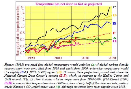
An early projection of the trend in TS in response to “global warming” was that of Hansen (1988), amplifying Hansen (1984) on quantification of climate sensitivity. In 1988, Hansen showed Congress a graph projecting rapid increases in TS to 2020 through “global warming” (Fig. 2):

Figure 2
Global temperature projections and outturns, 1988-2020


To what extent, then, has humankind warmed the world, and how much warmer will the world become if the current rate of increase in anthropogenic CO2 emissions continues? Estimating “climate sensitivity” – the magnitude of the change in TS after doubling CO2 concentration from the pre-industrial 278 parts per million to ~550 ppm – is the central question in the scientific debate about the climate. The official answer is given in IPCC (2007):

“It is very likely that anthropogenic greenhouse gas increases caused most of the observed increase in [TS] since the mid-20th century. … The equilibrium global average warming expected if carbon dioxide concentrations were to be sustained at 550 ppm is likely to be in the range 2-4.5 °C above pre-industrial values, with a best estimate of about 3 °C.”

Here as elsewhere the IPCC assigns a 90% confidence interval to “very likely”, rather than the customary 95% (two standard deviations). There is no good statistical basis for any such quantification, for the object to which it is applied is, in the formal sense, chaotic. The climate is “a complex, nonlinear, chaotic object” that defies long-run prediction of its future states (IPCC, 2001), unless the initial state of its millions of variables is known to a precision that is in practice unattainable, as Lorenz (1963; and see Giorgi, 2005) concluded in the celebrated paper that founded chaos theory –
“Prediction of the sufficiently distant future is impossible by any method, unless the present conditions are known exactly. In view of the inevitable inaccuracy and incompleteness of weather observations, precise, very-long-range weather forecasting would seem to be nonexistent.”  The Summary for Policymakers in IPCC (2007) says –“The CO2 radiative forcing increased by 20% in the last 10 years (1995-2005).”

Natural or anthropogenic CO2 in the atmosphere induces a “radiative forcing” ΔF, defined by IPCC (2001: ch.6.1) as a change in net (down minus up) radiant-energy flux at the tropopause in response to a perturbation. Aggregate forcing is natural (pre-1750) plus anthropogenic-era (post-1750) forcing. At 1990, aggregate forcing from CO2 concentration was ~27 W m–2 (Kiehl & Trenberth, 1997). From 1995-2005, CO2 concentration rose 5%, from 360 to 378 W m–2, with a consequent increase in aggregate forcing (from Eqn. 3 below) of ~0.26 W m–2, or <1%. That is one-twentieth of the value
stated by the IPCC. The absence of any definition of “radiative forcing” in the 2007 Summary led many to believe that the aggregate (as opposed to anthropogenic) effect of CO2 on TS had increased by 20% in 10 years. The IPCC – despite requests for correction – retained this confusing statement in its report.  Such solecisms throughout the IPCC’s assessment reports (including the insertion, after the scientists had completed their final draft, of a table in which four decimal points had been right-shifted so as to multiply tenfold the observed contribution of ice-sheets and glaciers to sea-level rise), combined with a heavy reliance upon computer models unskilled even in short-term projection, with initial values of key
variables unmeasurable and unknown, with advancement of multiple, untestable, non-Popperfalsifiable theories, with a quantitative assignment of unduly high statistical confidence levels to nonquantitative statements that are ineluctably subject to very large uncertainties, and, above all, with the now-prolonged failure of TS to rise as predicted (Figures 1, 2), raise questions about the reliability and hence policy-relevance of the IPCC’s central projections.

Dr. Rajendra Pachauri, chairman of the UN Intergovernmental Panel on Climate Change (IPCC), has recently said that the IPCC’s evaluation of climate sensitivity must now be revisited. This paper is a respectful contribution to that re-examination.

The IPCC’s method of evaluating climate sensitivity

We begin with an outline of the IPCC’s method of evaluating climate sensitivity. For clarity we will concentrate on central estimates. The IPCC defines climate sensitivity as equilibrium temperature change ΔTλ in response to all anthropogenic-era radiative forcings and consequent “temperature feedbacks” – further changes in TS that occur because TS has already changed in response to a forcing – arising in response to the doubling of pre-industrial CO2 concentration (expected later this century).  ΔTλ is, at its simplest, the product of three factors: the sum ΔF2x of all anthropogenic-era radiative forcings at CO2 doubling; the base or “no-feedbacks” climate sensitivity parameter κ; and the feedback
multiplier f, such that the final or “with-feedbacks” climate sensitivity parameter λ = κ f. Thus –

ΔTλ = ΔF2x κ f = ΔF2x λ, (1)
where f = (1 – bκ)–1, (2)

such that b is the sum of all climate-relevant temperature feedbacks. The definition of f in Eqn. (2) will be explained later. We now describe seriatim each of the three factors in ΔTλ: namely, ΔF2x, κ, and f.

1. Radiative forcing ΔFCO2, where (C/C0) is a proportionate increase in CO2 concentration, is given by several formulae in IPCC (2001, 2007). The simplest, following Myrhe (1998), is Eqn. (3) –

ΔFCO2 ≈ 5.35 ln(C/C0) ==> ΔF2xCO2 ≈ 5.35 ln 2 ≈ 3.708 W m–2. (3)

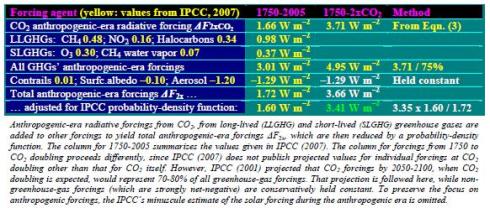
To ΔF2xCO2 is added the slightly net-negative sum of all other anthropogenic-era radiative forcings, calculated from IPCC values (Table 1), to obtain total anthropogenic-era radiative forcing ΔF2x at CO2 doubling (Eqn. 3). Note that forcings occurring in the anthropogenic era may not be anthropogenic.

Table 1
Evaluation of ΔF2x from the IPCC’s anthropogenic-era forcings


From the anthropogenic-era forcings summarized in Table 1, we obtain the first of the three factors –
ΔF2x ≈ 3.405 Wm–2. (4)

Continue to Part 2

Climate Sensitivity Reconsidered Part 2

A special report from Christopher Monckton of Brenchley to all Climate Alarmists, Consensus Theorists and Anthropogenic Global Warming Supporters

Continues from Part 1

2. The base or “no-feedbacks” climate sensitivity parameter κ, where ΔTκ is the response of TS to radiative forcings ignoring temperature feedbacks, ΔTλ is the response of TS to feedbacks as well as forcings, and b is the sum in W m–2 °K–1 of all individual temperature feedbacks, is –

κ = ΔTκ / ΔF2x °K W–1 m2, by definition; (5)
= ΔTλ / (ΔF2x + bΔTλ) °K W–1 m2. (6)

In Eqn. (5), ΔTκ, estimated by Hansen (1984) and IPCC (2007) as 1.2-1.3 °K at CO2 doubling, is the change in surface temperature in response to a tropopausal forcing ΔF2x, ignoring any feedbacks.  ΔTκ is not directly mensurable in the atmosphere because feedbacks as well as forcings are present.  Instruments cannot distinguish between them. However, from Eqn. (2) we may substitute 1 / (1 – bκ) for f in Eqn. (1), rearranging terms to yield a useful second identity, Eqn. (6), expressing κ in terms of ΔTλ, which is mensurable, albeit with difficulty and subject to great uncertainty (McKitrick, 2007).  IPCC (2007) does not mention κ and, therefore, provides neither error-bars nor a “Level of Scientific
Understanding” (the IPCC’s subjective measure of the extent to which enough is known about a variable to render it useful in quantifying climate sensitivity). However, its implicit value κ ≈ 0.313 °K W–1 m2, shown in Eqn. 7, may be derived using Eqns. 9-10 below, showing it to be the reciprocal of the estimated “uniform-temperature” radiative cooling response–

“Under these simplifying assumptions the amplification [f] of the global warming from a feedback parameter [b] (in W m–2 °C–1) with no other feedbacks operating is 1 / (1 –[bκ –1]), where [–κ –1] is the ‘uniform temperature’ radiative cooling response (of value approximately –3.2 W m–2 °C–1; Bony et al., 2006). If n independent feedbacks operate, [b] is replaced by (λ1 + λ 2+ … λ n).” (IPCC, 2007: ch.8, footnote).

Thus, κ ≈ 3.2–1 ≈ 0.313 °K W–1 m2. (7)

3. The feedback multiplier f is a unitless variable by which the base forcing is multiplied to take account of mutually-amplified temperature feedbacks. A “temperature feedback” is a change in TS that occurs precisely because TS has already changed in response to a forcing or combination of forcings.  An instance: as the atmosphere warms in response to a forcing, the carrying capacity of the space occupied by the atmosphere for water vapor increases near-exponentially in accordance with the Clausius-Clapeyron relation. Since water vapor is the most important greenhouse gas, the growth in its
concentration caused by atmospheric warming exerts an additional forcing, causing temperature to rise further. This is the “water-vapor feedback”. Some 20 temperature feedbacks have been described, though none can be directly measured. Most have little impact on temperature. The value of each feedback, the interactions between feedbacks and forcings, and the interactions between feedbacks and other feedbacks, are subject to very large uncertainties.

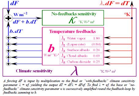
Each feedback, having been triggered by a change in atmospheric temperature, itself causes a temperature change. Consequently, temperature feedbacks amplify one another. IPCC (2007: ch.8) defines f in terms of a form of the feedback-amplification function for electronic circuits given in Bode (1945), where b is the sum of all individual feedbacks before they are mutually amplified:

f = (1 – bκ)–1 (8)
= ΔTλ / ΔTκ

Note the dependence of f not only upon the feedback-sum b but also upon κ –

ΔTλ = (ΔF + bΔTλ)κ
==> ΔTλ (1 – bκ) = ΔFκ
==> ΔTλ = ΔFκ(1 – bκ)–1
==> ΔTλ / ΔF = λ = κ(1 – bκ)–1 = κf
==> f = (1 – bκ)–1 ≈ (1 – b / 3.2)–1
==> κ ≈ 3.2–1 ≈ 0.313 °K W–1 m2. (9)

Equivalently, expressing the feedback loop as the sum of an infinite series,

ΔTλ = ΔFκ + ΔFκ 2b + ΔFκ 2b2 + …
= ΔFκ(1 + κb + κb2 + …)
= ΔFκ(1 – κb)–1
= ΔFκf
==> λ = ΔTλ /ΔF = κf (10)

Figure 3
Bode (1945) feedback amplification schematic


For the first time, IPCC (2007) quantifies the key individual temperature feedbacks summing to b:
“In AOGCMs, the water vapor feedback constitutes by far the strongest feedback, with a multi-model mean and standard deviation … of 1.80 ± 0.18 W m–2 K–1, followed by the negative lapse rate feedback (–0.84 ± 0.26 W m–2 K–1) and the surface albedo feedback (0.26 ± 0.08 W m–2 K–1). The cloud feedback mean is 0.69 W m–2 K–1 with a very large inter-model spread of ±0.38 W m–2K–1.” (Soden & Held, 2006).

To these we add the CO2 feedback, which IPCC (2007, ch.7) separately expresses not as W m–2 °K–1 but as concentration increase per CO2 doubling: [25, 225] ppmv, central estimate q = 87 ppmv. Where p is concentration at first doubling, the proportionate increase in atmospheric CO2 concentration from the CO2 feedback is o = (p + q) / p = (556 + 87) / 556 ≈ 1.16. Then the CO2 feedback is –λCO2 = z ln(o) / dTλ ≈ 5.35 ln(1.16) / 3.2 ≈ 0.25 Wm–2 K–1. (11) The CO2 feedback is added to the previously-itemized feedbacks to complete the feedback-sum b:

b = 1.8 – 0.84 + 0.26 + 0.69 + 0.25 ≈ 2.16 Wm–2 ºK–1, (12)

so that, where κ = 0.313, the IPCC’s unstated central estimate of the value of the feedback factor f is at the lower end of the range f = 3-4 suggested in Hansen et al. (1984) –

f = (1 – bκ)–1 ≈ (1 – 2.16 x 0.313)–1 ≈ 3.077. (13)

Final climate sensitivity ΔTλ, after taking account of temperature feedbacks as well as the forcings that triggered them, is simply the product of the three factors described in Eqn. (1), each of which we have briefly described above. Thus, at CO2 doubling, –

ΔTλ = ΔF2x κ f ≈ 3.405 x 0.313 x 3.077 ≈ 3.28 °K (14)

IPCC (2007) gives dTλ on [2.0, 4.5] ºK at CO2 doubling, central estimate dTλ ≈ 3.26 °K, demonstrating that the IPCC’s method has been faithfully replicated. There is a further checksum, –

ΔTκ = ΔTλ / f = κ ΔF2x = 0.313 x 3.405 ≈ 1.1 °K, (15)

sufficiently close to the IPCC’s estimate ΔTκ ≈ 1.2 °K, based on Hansen (1984), who had estimated a range 1.2-1.3 °K based on his then estimate that the radiative forcing ΔF2xCO2 arising from a CO2 doubling would amount to 4.8 W m–2, whereas the IPCC’s current estimate is ΔF2xCO2 = 3.71 W m–2 (see Eqn. 2), requiring a commensurate reduction in ΔTκ that the IPCC has not made.  A final checksum is provided by Eqn. (5), giving a value identical to that of the IPCC at Eqn (7):

κ = ΔTλ / (ΔF2x + bΔTλ)
≈ 3.28 / (3.405 + 2.16 x 3.28)
≈ 0.313 °K W–1 m2. (16)

Having outlined the IPCC’s methodology, we proceed to re-evaluate each of the three factors in dTλ.  None of these three factors is directly mensurable. For this and other reasons, it is not possible to obtain climate sensitivity numerically using general-circulation models: for, as Akasofu (2008) has pointed out, climate sensitivity must be an input to any such model, not an output from it.  In attempting a re-evaluation of climate sensitivity, we shall face the large uncertainties inherent in the climate object, whose complexity, non-linearity, and chaoticity present formidable initial-value and boundary-value problems. We cannot measure total radiative forcing, with or without temperature feedbacks, because radiative and non-radiative atmospheric transfer processes combined with seasonal, latitudinal, and altitudinal variabilities defeat all attempts at reliable measurement. We cannot even measure changes in TS to within a factor of two (McKitrick, 2007).

Even satellite-based efforts at assessing total energy-flux imbalance for the whole Earth-troposphere system are uncertain. Worse, not one of the individual forcings or feedbacks whose magnitude is essential to an accurate evaluation of climate sensitivity is mensurable directly, because we cannot distinguish individual forcings or feedbacks one from another in the real atmosphere, we can only guess at the interactions between them, and we cannot even measure the relative contributions of all forcings and of all feedbacks to total radiative forcing. Therefore we shall adopt two approaches:
theoretical demonstration (where possible); and empirical comparison of certain outputs from the models with observation to identify any significant inconsistencies.

Radiative forcing ΔF2x reconsidered

We take the second approach with ΔF2x. Since we cannot measure any individual forcing directly in the atmosphere, the models draw upon results of laboratory experiments in passing sunlight through chambers in which atmospheric constituents are artificially varied; such experiments are, however, of limited value when translated into the real atmosphere, where radiative transfers and non-radiative transports (convection and evaporation up, advection along, subsidence and precipitation down), as well as altitudinal and latitudinal asymmetries, greatly complicate the picture. Using these laboratory values, the models attempt to produce latitude-versus-altitude plots to display the characteristic
signature of each type of forcing. The signature or fingerprint of anthropogenic greenhouse-gas forcing, as predicted by the models on which the IPCC relies, is distinct from that of any other forcing, in that the models project that the rate of change in temperature in the tropical mid-troposphere – the region some 6-10 km above the surface – will be twice or thrice the rate of change at the surface (Figure 4):

Figure 4
Temperature fingerprints of five forcings Modeled zonal


The fingerprint of anthropogenic greenhouse-gas forcing is a distinctive “hot-spot” in the tropical midtroposphere.
Figure 4 shows altitude-vs.-latitude plots from four of the IPCC’s models:

Figure 5
Fingerprints of anthropogenic warming projected by four models


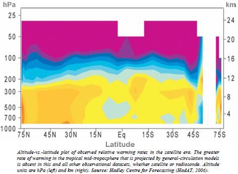
However, as Douglass et al. (2004) and Douglass et al. (2007) have demonstrated, the projected
fingerprint of anthropogenic greenhouse-gas warming in the tropical mid-troposphere is not observed
in reality. Figure 6 is a plot of observed tropospheric rates of temperature change from the Hadley
Center for Forecasting. In the tropical mid-troposphere, at approximately 300 hPa pressure, the model projected
fingerprint of anthropogenic greenhouse warming is absent from this and all other observed
records of temperature changes in the satellite and radiosonde eras:

Continue to Part 3

Climate Sensitivity Reconsidered Part 3

A special report from Christopher Monckton of Brenchley to all Climate Alarmists, Consensus Theorists and Anthropogenic Global Warming Supporters

Continues from Part 2

Figure 6
The absent fingerprint of anthropogenic greenhouse warming


None of the temperature datasets for the tropical surface and mid-troposphere shows the strong differential warming rate predicted by the IPCC’s models. Thorne et al. (2007) suggested that the absence of the mid-tropospheric warming might be attributable to uncertainties in the observed record: however, Douglass et al. (2007) responded with a detailed statistical analysis demonstrating that the absence of the projected degree of warming is significant in all observational datasets.  Allen et al. (2008) used upper-atmosphere wind speeds as a proxy for temperature and concluded that
the projected greater rate of warming at altitude in the tropics is occurring in reality. However, satellite records, such as the RSS temperature trends at varying altitudes, agree with the radiosondes that the warming differential is not occurring: they show that not only absolute temperatures but also warming rates decline with altitude.  There are two principal reasons why the models appear to be misrepresenting the tropical atmosphere so starkly. First, the concentration of water vapor in the tropical lower troposphere is already so great that there is little scope for additional greenhouse-gas forcing. Secondly, though the models assume that the concentration of water vapor will increase in the tropical mid-troposphere as the space occupied by the atmosphere warms, advection transports much of the additional water vapor poleward
from the tropics at that altitude.

Since the great majority of the incoming solar radiation incident upon the Earth strikes the tropics, any reduction in tropical radiative forcing has a disproportionate effect on mean global forcings. On the basis of Lindzen (2007), the anthropogenic-ear radiative forcing as established in Eqn. (3) are divided by 3 to take account of the observed failure of the tropical mid-troposphere to warm as projected by the models –

ΔF2x ≈ 3.405 / 3 ≈ 1.135 Wm–2. (17)

The “no-feedbacks” climate sensitivity parameter κ reconsidered The base climate sensitivity parameter κ is the most influential of the three factors of ΔTλ: for the final or “with-feedbacks” climate sensitivity parameter λ is the product of κ and the feedback factor f, which is itself dependent not only on the sum b of all climate-relevant temperature feedbacks but also on κ.  Yet κ has received limited attention in the literature. In IPCC (2001, 2007) it is not mentioned.
However, its value may be deduced from hints in the IPCC’s reports. IPCC (2001, ch. 6.1) says:

“The climate sensitivity parameter (global mean surface temperature response ΔTS to the radiative forcing
ΔF) is defined as ΔTS / ΔF = λ {6.1} (Dickinson, 1982; WMO, 1986; Cess et al., 1993). Equation {6.1} is defined for the transition of the surface-troposphere system from one equilibrium state to another in response to an externally imposed radiative perturbation. In the one-dimensional radiative-convective models, wherein the concept was first initiated, λ is a nearly invariant parameter (typically, about 0.5 °K W−1 m2; Ramanathan et al., 1985) for a variety of radiative forcings, thus introducing the notion of a possible universality of the relationship between forcing and response.”

Since λ = κf = κ(1 – bκ)–1 (Eqns. 1, 2), where λ = 0.5 °K W–1 m2 and b ≈ 2.16 W m–2 °K–1 (Eqn. 12), it is simple to calculate that, in 2001, one of the IPCC’s values for f was 2.08. Thus the value f = 3.077 in IPCC (2007) represents a near-50% increase in the value of f in only five years. Where f = 2.08, κ = λ / f ≈ 0.5 / 2.08 ≈ 0.24 °K W–1 m2, again substantially lower than the value implicit in IPCC (2007).

Some theory will, therefore, be needed.

The fundamental equation of radiative transfer at the emitting surface of an astronomical body, relating changes in radiant-energy flux to changes in temperature, is the Stefan-Boltzmann equation – F = ε σ T4 W m–2, (18)
where F is radiant-energy flux at the emitting surface; ε is emissivity, set at 1 for a blackbody that absorbs and emits all irradiance reaching its emitting surface (by Kirchhoff’s law of radiative transfer, absorption and emission are equal and simultaneous), 0 for a white body that reflects all irradiance, and (0, 1) for a graybody that partly absorbs/emits and partly reflects; and σ ≈ 5.67 x 10⁻⁸ is the Stefan-Boltzmann constant.  Differentiating Eqn. (18) gives –

κ = dT / dF = (dF / dT)–1 = (4 ε σ T3)–1 °K W–1 m2. (19) Outgoing radiation from the Earth’s surface is chiefly in the near-infrared. Its peak wavelength λmax is determined solely by the temperature of the emitting surface in accordance with Wien’s Displacement Law, shown in its simplest form in Eqn. (20):

λmax = 2897 / TS = 2897 / 288 ≈ 10 μm. (20)

Since the Earth/troposphere system is a blackbody with respect to the infrared radiation that Eqn. (20) shows we are chiefly concerned with, we will not introduce any significant error if ε = 1, giving the blackbody form of Eqn. (19) –

κ = dT / dF = (4 σ T3)–1 °K W–1 m2. (21)

At the Earth’s surface, TS ≈ 288 °K, so that κS ≈ 0.185 °K W–1 m2. At the characteristic-emission level, ZC, the variable altitude at which incoming and outgoing radiative fluxes balance, TC ≈ 254 °K, so that κC ≈ 0.269 °K W–1 m2. The value κC ≈ 0.24, derived from the typical final-sensitivity value λ = 0.5 given in IPCC (2001), falls between the surface and characteristic-emission values for κ.

However, the IPCC, in its evaluation of κ, does not follow the rule that in the Stefan-Boltzmann equation the temperature and radiant-energy flux must be taken at the same level of the atmosphere.  The IPCC’s value for κ is dependent upon temperature at the surface and radiant-energy flux at the tropopause, so that its implicit value κ ≈ 0.313 °K W–1 m2 is considerably higher than either κS or κC.  IPCC (2007) cites Hansen et al. (1984), who say –

“Our three-dimensional global climate model yields a warming of ~4 ºC for … doubled CO2. This indicates a net feedback factor f = 3-4, because [the forcing at CO2 doubling] would cause the earth’s surface temperature to warm 1.2-1.3 ºC to restore radiative balance with space, if other factors remained unchanged.”

Hansen says dF2x is equivalent to a 2% increase in incoming total solar irradiance (TSI). Top-ofatmosphere
TSI S ≈ 1368 W m2, albedo α = 0.31, and Earth’s radius is r. Then, at the characteristic
emission level ZC,

FC = S(1 – α)(πr2 / 4πr2) ≈ 1368 x 0.69 x (1/4) ≈ 236 Wm–2. (22)

Thus a 2% increase in FC is equivalent to 4.72 W m–2, rounded up by Hansen to 4.8 W m–2, implying that κ ≈ 1.25 / 4.8 ≈ 0.260 °K W–1 m2. However, Hansen, in his Eqn. {14}, prefers 0.29 Wm–2.  Bony et al. (2006), also cited by IPCC (2007), do not state a value for κ. However, they say – “The Planck feedback parameter [equivalent to κ –1] is negative (an increase in temperature enhances the long-wave emission to space and thus reduces R [the Earth’s radiation budget]), and its typical value for the earth’s atmosphere, estimated from GCM calculations (Colman 2003; Soden and Held 2006), is ~3.2 W m2 ºK–1 (a value of ~3.8 W m2 ºK–1 is obtained by defining [κ –1] simply as 4σT3, by equating the global
mean outgoing long-wave radiation to σT4 and by assuming an emission temperature of 255 ºK).” Bony takes TC ≈ 255 °K and FC ≈ 235 W m–2 at ZC as the theoretical basis for the stated prima facie value κ –1 ≈ TC / 4FC ≈ 3.8 W m2 ºK–1, so that κ ≈ 0.263 ºK W–1 m2, in very close agreement with Hansen. However, Bony cites two further papers, Colman (2003) and Soden & Held (2006), as justification for the value κ –1 ≈ 3.2 W m2 ºK–1, so that κ ≈ 0.313 ºK W–1 m2.  Colman (2003) does not state a value for κ, but cites Hansen et al. (1984), rounding up the value κ ≈ 0.260 °K W–1 m2 to 0.3 °K W–1 m2 – “The method used assumes a surface temperature increase of 1.2 °K with only the CO2 forcing and the
‘surface temperature’ feedback operating (value originally taken from Hansen et al. 1984).”

Soden & Held (2006) likewise do not declare a value for κ. However, we may deduce their implicit central estimate κ ≈ 1 / 4 ≈ 0.250 °K W–1 m2 from the following passage – “The increase in opacity due to a doubling of CO2 causes [the characteristic emission level ZC] to rise by ~150 meters. This results in a reduction in the effective temperature of the emission across the tropopause by ~(6.5K/km)(150 m) ≈ 1 K, which converts to 4 W m–2 using the Stefan-Boltzmann law.”  Thus the IPCC cites only two papers that cite two others in turn. None of these papers provides any theoretical or empirical justification for a value as high as the κ ≈ 0.313 °K W–1 m2 chosen by the IPCC.

Kiehl (1992) gives the following method, where FC is total flux at ZC:

κS = TS / (4FC) ≈ 288 / (4 x 236) ≈ 0.305 °K W–1 m2. (23)

Hartmann (1994) echoes Kiehl’s method, generalizing it to any level J of an n-level troposphere thus:

κJ = TJ / (4FC)
= TJ / [S(1 – α)]
≈ TJ / [1368(1 – 0.31)] ≈ TJ / 944 °K W–1 m2. (24)

Table 2 summarizes the values of κ evident in the cited literature, with their derivations, minores priores. The greatest value, chosen in IPCC (2007), is 30% above the least, chosen in IPCC (2001).  However, because the feedback factor f depends not only upon the feedback-sum b ≈ 2.16 W m–2 °K–1  but also upon κ, the 30% increase in κ nearly doubles final climate sensitivity:

Table 2
Values of the “no-feedbacks” climate sensitivity parameter κ


The value of κ cannot be deduced by observation, because temperature feedbacks are present and cannot be separately measured. However, it is possible to calculate κ using Eqn. (6), provided that the temperature change ΔTλ, radiative forcings ΔF2x, and feedback-sum b over a given period are known.  The years 1980 and 2005 will be compared, giving a spread of a quarter of a century. We take the feedback-sum b = 2.16 W m–2 °K–1 and begin by establishing values for ΔF and ΔT:  CO2 concentration: 338.67 ppmv 378.77 ppmv ΔF = 5.35 ln (378.77/338.67) = 0.560 W m–2 Anomaly in TS: 0.144 °K 0.557 °K ΔT = 0.412 °K (NCDC) Anomaly halved: ΔT = 0.206 °K (McKitrick) (25) CO2 concentrations are the annual means from 100 stations (Keeling & Whorf, 2004, updated). TS values are NCDC annual anomalies, as five-year means centered on 1980 and 2005 respectively. Now, depending on whether the NCDC or implicit McKitrick value is correct, κ may be directly evaluated:

NCDC: κ = ΔT / (ΔF + bΔT) = 0.412 / (0.560 + 2.16 x 0.412) = 0.284 °KW–1 m2
McKitrick: κ = ΔT / (ΔF + bΔT) = 0.206 / (0.599 + 2.16 x 0.206) = 0.197 °KW–1 m2
Mean: κ = (0.284 + 0.197) / 2 = 0.241 °KW–1 m2 (26)

We assume that Chylek (2008) is right to find transient and equilibrium climate sensitivity near identical; that all of the warming from 1980-2005 was anthropogenic; that the IPCC’s values for forcings and feedbacks are correct; and, in line 2, that McKitrick is right that the insufficiently corrected heat-island effect of rapid urbanization since 1980 has artificially doubled the true rate of temperature increase in the major global datasets.

With these assumptions, κ is shown to be less, and perhaps considerably less, than the value implicit in IPCC (2007). The method of finding κ shown in Eqn. (24), which yields a value very close to that of IPCC (2007), is such that progressively smaller forcing increments would deliver progressively larger temperature increases at all levels of the atmosphere, contrary to the laws of thermodynamics and to the Stefan-Boltzmann radiative-transfer equation (Eqn. 18), which mandate the opposite. It is accordingly necessary to select a value for κ that falls well below the IPCC’s value. Dr. David Evans (personal communication, 2007) has calculated that the characteristic-emission-level value of κ should be diminished by ~10% to allow for the non-uniform latitudinal distribution of incoming solar radiation, giving a value near-identical to that in Eqn. (26), and to that implicit in IPCC (2001), thus –

κ = 0.9TC / [S(1 – α)]
≈ 0.9 x 254 / [1368(1 – 0.31)] ≈ 0.242 °K W–1 m2 (27)

The feedback factor f reconsidered

The feedback factor f accounts for two-thirds of all radiative forcing in IPCC (2007); yet it is not expressly quantified, and no “Level Of Scientific Understanding” is assigned either to f or to the two variables b and κ upon which it is dependent.
Several further difficulties are apparent. Not the least is that, if the upper estimates of each of the climate-relevant feedbacks listed in IPCC (2007) are summed, an instability arises. The maxima are –

Water vapor feedback 1.98 W m–2 K–1
Lapse rate feedback –0.58 W m–2 K–1
Surface albedo feedback 0.34 W m–2 K–1
Cloud albedo feedback 1.07 W m–2 K–1
CO2 feedback 0.57 W m–2 K–1
Total feedbacks b 3.38 Wm–2 K–1 (28)

Continue to Part 4

Climate Sensitivity Reconsidered Part 4

A special report from Christopher Monckton of Brenchley to all Climate Alarmists, Consensus Theorists and Anthropogenic Global Warming Supporters

Continues from Part 3

Since the equation [f = (1 – bκ)–1] → ∞ as b → [κ–1 = 3.2 W m–2 K–1], the feedback-sum b cannot exceed 3.2 W m–2 K–1 without inducing a runaway greenhouse effect. Since no such effect has been observed or inferred in more than half a billion years of climate, since the concentration of CO2 in the Cambrian atmosphere approached 20 times today’s concentration, with an inferred mean global surface temperature no more than 7 °K higher than today’s (Figure 7), and since a feedback-induced runaway greenhouse effect would occur even in today’s climate where b >= 3.2 W m–2 K–1 but has not occurred, the IPCC’s high-end estimates of the magnitude of individual temperature feedbacks are very likely to be excessive, implying that its central estimates are also likely to be excessive.

Figure 7
Fluctuating CO2 but stable temperature for 600m years
Millions of years before present


Since absence of correlation necessarily implies absence of causation, Figure 7 confirms what the recent temperature record implies: the causative link between changes in CO2 concentration and changes in temperature cannot be as strong as the IPCC has suggested. The implications for climate sensitivity are self-evident. Figure 7 indicates that in the Cambrian era, when CO2 concentration was ~25 times that which prevailed in the IPCC’s reference year of 1750, the temperature was some 8.5 °C higher than it was in 1750. Yet the IPCC’s current central estimate is that a mere doubling of CO2 concentration compared with 1750 would increase temperature by almost 40% of the increase that is thought to have arisen in geological times from a 20-fold increase in CO2 concentration (IPCC, 2007).

How could such over statements of individual feedbacks have arisen? Not only is it impossible to obtain empirical confirmation of the value of any feedback by direct measurement; it is questionable whether the feedback equation presented in Bode (1945) is appropriate to the climate. That equation was intended to model feedbacks in linear electronic circuits: yet many temperature feedbacks – the water vapor and CO2 feedbacks, for instance – are non-linear. Feedbacks, of course, induce non-linearity in linear objects: nevertheless, the Bode equation is valid only for objects whose initial state is linear. The climate is not a linear object: nor are most of the climate-relevant temperature feedbacks linear. The
water-vapor feedback is an interesting instance of the non-linearity of temperature feedbacks. The increase in water-vapor concentration as the space occupied by the atmosphere warms is near exponential; but the forcing effect of the additional water vapor is logarithmic. The IPCC’s use of the Bode equation, even as a simplifying assumption, is accordingly questionable.

IPCC (2001: ch.7) devoted an entire chapter to feedbacks, but without assigning values to each feedback that was mentioned. Nor did the IPCC assign a “Level of Scientific Understanding” to each feedback, as it had to each forcing. In IPCC (2007), the principal climate-relevant feedbacks are quantified for the first time, but, again, no Level of Scientific Understanding” is assigned to them, even though they account for more than twice as much forcing as the greenhouse-gas and other anthropogenic-era forcings to which “Levels of Scientific Understanding” are assigned.

Now that the IPCC has published its estimates of the forcing effects of individual feedbacks for the first time, numerous papers challenging its chosen values have appeared in the peer-reviewed literature.  Notable among these are Wentz et al. (2007), who suggest that the IPCC has failed to allow for two thirds of the cooling effect of evaporation in its evaluation of the water vapor-feedback; and Spencer (2007), who points out that the cloud-albedo feedback, regarded by the IPCC as second in magnitude only to the water-vapor feedback, should in fact be negative rather than strongly positive.
It is, therefore, prudent and conservative to restore the values κ ≈ 0.24 and f ≈ 2.08 that are derivable from IPCC (2001), adjusting the values a little to maintain consistency with Eqn. (27). Accordingly, our revised central estimate of the feedback multiplier f is –

f = (1 – bκ)–1 ≈ (1 – 2.16 x 0.242)–1 ≈ 2.095 (29)

Final climate sensitivity

Substituting in Eqn. (1) the revised values derived for the three factors in ΔTλ, our re-evaluated central estimate of climate sensitivity is their product –

ΔTλ = ΔF2x κ f ≈ 1.135 x 0.242 x 2.095 ≈ 0.58 °K (30)

Theoretically, empirically, and in the literature that we have extensively cited, each of the values we have chosen as our central estimate is arguably more justifiable – and is certainly no less justifiable – than the substantially higher value selected by the IPCC. Accordingly, it is very likely that in response to a doubling of pre-industrial carbon dioxide concentration TS will rise not by the 3.26 °K suggested by the IPCC, but by <1 °K.

Discussion

We have set out and then critically examined a detailed account of the IPCC’s method of evaluating climate sensitivity. We have made explicit the identities, interrelations, and values of the key variables, many of which the IPCC does not explicitly describe or quantify. The IPCC’s method does not provide a secure basis for policy-relevant conclusions. We now summarize some of its defects The IPCC’s methodology relies unduly – indeed, almost exclusively – upon numerical analysis, even where the outputs of the models upon which it so heavily relies are manifestly and significantly at variance with theory or observation or both. Modeled projections such as those upon which the IPCC’s entire case rests have long been proven impossible when applied to mathematically-chaotic objects, such as the climate, whose initial state can never be determined to a sufficient precision. For a similar reason, those of the IPCC’s conclusions that are founded on probability distributions in the chaotic climate object are unsafe.

Not one of the key variables necessary to any reliable evaluation of climate sensitivity can be measured empirically. The IPCC’s presentation of its principal conclusions as though they were near-certain is accordingly unjustifiable. We cannot even measure mean global surface temperature anomalies to within a factor of 2; and the IPCC’s reliance upon mean global temperatures, even if they could be correctly evaluated, itself introduces substantial errors in its evaluation of climate sensitivity.

The IPCC overstates the radiative forcing caused by increased CO2 concentration at least threefold because the models upon which it relies have been programmed fundamentally to misunderstand the difference between tropical and extra-tropical climates, and to apply global averages that lead to error. The IPCC overstates the value of the base climate sensitivity parameter for a similar reason. Indeed, its methodology would in effect repeal the fundamental equation of radiative transfer (Eqn. 18), yielding the impossible result that at every level of the atmosphere ever-smaller forcings would induce ever greater temperature increases, even in the absence of any temperature feedbacks.

The IPCC overstates temperature feedbacks to such an extent that the sum of the high-end values that it has now, for the first time, quantified would cross the instability threshold in the Bode feedback equation and induce a runaway greenhouse effect that has not occurred even in geological times despite CO2 concentrations almost 20 times today’s, and temperatures up to 7 ºC higher than today’s.  The Bode equation, furthermore, is of questionable utility because it was not designed to model feedbacks in non-linear objects such as the climate. The IPCC’s quantification of temperature
feedbacks is, accordingly, inherently unreliable. It may even be that, as Lindzen (2001) and Spencer (2007) have argued, feedbacks are net-negative, though a more cautious assumption has been made in this paper.

It is of no little significance that the IPCC’s value for the coefficient in the CO2 forcing equation depends on only one paper in the literature; that its values for the feedbacks that it believes account for two-thirds of humankind’s effect on global temperatures are likewise taken from only one paper; and that its implicit value of the crucial parameter κ depends upon only two papers, one of which had been written by a lead author of the chapter in question, and neither of which provides any theoretical or empirical justification for a value as high as that which the IPCC adopted.

The IPCC has not drawn on thousands of published, peer-reviewed papers to support its central estimates for the variables from which climate sensitivity is calculated, but on a handful. On this brief analysis, it seems that no great reliance can be placed upon the IPCC’s central estimates of climate sensitivity, still less on its high-end estimates. The IPCC’s assessments, in their current state, cannot be said to be “policy-relevant”. They provide no justification for taking the very costly and
drastic actions advocated in some circles to mitigate “global warming”, which Eqn. (30) suggests will be small (<1 °C at CO2 doubling), harmless, and beneficial.

Conclusion

Even if global temperature has risen, it has risen in a straight line at a natural 0.5 °C/century for 300 years since the Sun recovered from the Maunder Minimum, long before we could have had any influence (Akasofu, 2008).  Even if warming had sped up, now temperature is 7C below most of the past 500m yrs; 5C below all 4 recent inter-glacials; and up to 3C below the Bronze Age, Roman & mediaeval optima (Petit et al., 1999; IPCC, 1990).

Even if today’s warming were unprecedented, the Sun is the probable cause. It was more active in the past 70 years than in the previous 11,400 (Usoskin et al., 2003; Hathaway et al., 2004; IAU, 2004; Solanki et al., 2005).  Even if the sun were not to blame, the UN’s climate panel has not shown that humanity is to blame. CO2 occupies only one-ten-thousandth more of the atmosphere today than it did in 1750 (Keeling & Whorf, 2004).

Even if CO2 were to blame, no “runaway greenhouse” catastrophe occurred in the Cambrian era, when there was ~20 times today’s concentration in the air. Temperature was just 7 C warmer than today (IPCC, 2001).  Even if CO2 levels had set a record, there has been no warming since 1998. For 7 years, temperatures have fallen. The Jan 2007-Jan 2008 fall was the steepest since 1880 (GISS; Hadley; NCDC; RSS; UAH: all 2008).

Even if the planet were not cooling, the rate of warming is far less than the UN imagines. It would be too small to cause harm. There may well be no new warming until 2015, if then (Keenlyside et al., 2008).  Even if warming were harmful, humankind’s effect is minuscule. “The observed changes may be natural” (IPCC, 2001; cf. Chylek et al., 2008; Lindzen, 2007; Spencer, 2007; Wentz et al., 2007; Zichichi, 2007; etc.).  Even if our effect were significant, the UN’s projected human fingerprint – tropical mid-troposphere warming at thrice the surface rate – is absent (Douglass et al., 2004, 2007; Lindzen, 2001, 2007; Spencer, 2007).

Even if the human fingerprint were present, climate models cannot predict the future of the complex, chaotic climate unless we know its initial state to an unattainable precision (Lorenz, 1963; Giorgi, 2005; IPCC, 2001).  Even if computer models could work, they cannot predict future rates of warming. Temperature response to atmospheric greenhouse-gas enrichment is an input to the computers, not an output from them (Akasofu, 2008).  Even if the UN’s imagined high “climate sensitivity” to CO2 were right, disaster would not be likely to follow. The peer-reviewed literature is near-unanimous in not predicting climate catastrophe (Schulte, 2008).

Even if Al Gore were right that harm might occur, “the Armageddon scenario he depicts is not based on any scientific view”. Sea level may rise 1 ft to 2100, not 20 ft (Burton, J., 2007; IPCC, 2007; Moerner, 2004).  Even if Armageddon were likely, scientifically-unsound precautions are already starving millions as biofuels, a “crime against humanity”, pre-empt agricultural land, doubling staple cereal prices in a year. (UNFAO, 2008).  Even if precautions were not killing the poor, they would work no better than the “precautionary” ban on DDT, which killed 40 million children before the UN at last ended it (Dr. Arata Kochi, UN malaria program, 2006).

Even if precautions might work, the strategic harm done to humanity by killing the world’s poor and destroying the economic prosperity of the West would outweigh any climate benefit (Henderson, 2007; UNFAO, 2008).  Even if the climatic benefits of mitigation could outweigh the millions of deaths it is causing, adaptation as and if necessary would be far more cost-effective and less harmful (all economists except Stern, 2006).  Even if mitigation were as cost-effective as adaptation, the public sector – which emits twice as much carbon to do a given thing as the private sector – must cut its own size by half before it preaches to us (Friedman, 1993).

In short, we must get the science right, or we shall get the policy wrong. If the concluding equation in this analysis (Eqn. 30) is correct, the IPCC’s estimates of climate sensitivity must have been very much exaggerated. There may, therefore, be a good reason why, contrary to the projections of the models on which the IPCC relies, temperatures have not risen for a decade and have been falling since the phase transition in global temperature trends that occurred in late 2001. Perhaps real-world climate sensitivity is very much below the IPCC’s estimates. Perhaps, therefore, there is no “climate crisis” at all. At present, then, in policy terms there is no case for doing anything. The correct policy approach to a non-problem
is to have the courage to do nothing.

For a copy of this report on PDF format and a full list of references, please click here.

Daftar Akun Bandar Togel Resmi dengan Hadiah 4D 10 Juta Tahun 2024

Togel resmi adalah langkah penting bagi para penggemar togel yang ingin menikmati permainan dengan aman dan terpercaya. Tahun 2024 menawarkan berbagai kesempatan menarik, termasuk hadiah 4D sebesar 10 juta rupiah yang bisa Anda menangkan. Anda perlu mendaftar akun di Daftar Togel yang menawarkan hadiah tersebut. Proses pendaftaran biasanya sederhana dan melibatkan pengisian formulir dengan informasi pribadi Anda serta verifikasi data untuk memastikan keamanan transaksi. Setelah akun Anda selasai terdaftar, Anda dapat berpartisipasi dalam berbagai permainan togel berbagai fitur yang disediakan oleh situs togel terbesar.

Bermain di Link Togel memungkinkan Anda memasang taruhan dengan minimal 100 perak, sehingga semua kalangan bisa ikut serta. Meskipun taruhan rendah, Anda tetap bisa memenangkan hadiah besar dan mendapatkan bonus. Untuk mulai bermain, Anda harus mendaftar terlebih dahulu.

Bagi pemain togel yang ingin menikmati diskon terbesar, mendaftar di situs togel online terpercaya adalah langkah yang tepat. Bo Togel Hadiah 2d 200rb tidak hanya memberikan jaminan keamanan dalam bertransaksi, tetapi juga menawarkan berbagai diskon untuk jenis taruhan tertentu. Diskon yang besar ini memungkinkan pemain untuk menghemat lebih banyak dan memasang taruhan dalam jumlah yang lebih banyak. Dengan begitu, peluang untuk mendapatkan hadiah juga semakin tinggi, sekaligus memastikan bahwa setiap taruhan dilakukan di situs yang aman dan resmi.

Link Slot Gacor Terpercaya untuk Menang Setiap Hari

Slot gacor hari ini menjadi incaran para pemain Link Slot Gacor yang ingin menikmati peluang jackpot besar hanya dengan menggunakan modal kecil, sehingga mereka bisa merasakan pengalaman bermain yang lebih menyenangkan dan penuh keuntungan.

Related Links:

Togel178

Pedetogel

Sabatoto

Togel279

Togel158

Colok178

Novaslot88

Lain-Lain

Partner Links