A special report from Christopher Monckton of Brenchley to all Climate Alarmists, Consensus Theorists and Anthropogenic Global Warming Supporters
Continues from Part 1
2. The base or “no-feedbacks” climate sensitivity parameter κ, where ΔTκ is the response of TS to radiative forcings ignoring temperature feedbacks, ΔTλ is the response of TS to feedbacks as well as forcings, and b is the sum in W m–2 °K–1 of all individual temperature feedbacks, is –
κ = ΔTκ / ΔF2x °K W–1 m2, by definition; (5)
= ΔTλ / (ΔF2x + bΔTλ) °K W–1 m2. (6)
In Eqn. (5), ΔTκ, estimated by Hansen (1984) and IPCC (2007) as 1.2-1.3 °K at CO2 doubling, is the change in surface temperature in response to a tropopausal forcing ΔF2x, ignoring any feedbacks. ΔTκ is not directly mensurable in the atmosphere because feedbacks as well as forcings are present. Instruments cannot distinguish between them. However, from Eqn. (2) we may substitute 1 / (1 – bκ) for f in Eqn. (1), rearranging terms to yield a useful second identity, Eqn. (6), expressing κ in terms of ΔTλ, which is mensurable, albeit with difficulty and subject to great uncertainty (McKitrick, 2007). IPCC (2007) does not mention κ and, therefore, provides neither error-bars nor a “Level of Scientific
Understanding” (the IPCC’s subjective measure of the extent to which enough is known about a variable to render it useful in quantifying climate sensitivity). However, its implicit value κ ≈ 0.313 °K W–1 m2, shown in Eqn. 7, may be derived using Eqns. 9-10 below, showing it to be the reciprocal of the estimated “uniform-temperature” radiative cooling response–
“Under these simplifying assumptions the amplification [f] of the global warming from a feedback parameter [b] (in W m–2 °C–1) with no other feedbacks operating is 1 / (1 –[bκ –1]), where [–κ –1] is the ‘uniform temperature’ radiative cooling response (of value approximately –3.2 W m–2 °C–1; Bony et al., 2006). If n independent feedbacks operate, [b] is replaced by (λ1 + λ 2+ … λ n).” (IPCC, 2007: ch.8, footnote).
Thus, κ ≈ 3.2–1 ≈ 0.313 °K W–1 m2. (7)
3. The feedback multiplier f is a unitless variable by which the base forcing is multiplied to take account of mutually-amplified temperature feedbacks. A “temperature feedback” is a change in TS that occurs precisely because TS has already changed in response to a forcing or combination of forcings. An instance: as the atmosphere warms in response to a forcing, the carrying capacity of the space occupied by the atmosphere for water vapor increases near-exponentially in accordance with the Clausius-Clapeyron relation. Since water vapor is the most important greenhouse gas, the growth in its
concentration caused by atmospheric warming exerts an additional forcing, causing temperature to rise further. This is the “water-vapor feedback”. Some 20 temperature feedbacks have been described, though none can be directly measured. Most have little impact on temperature. The value of each feedback, the interactions between feedbacks and forcings, and the interactions between feedbacks and other feedbacks, are subject to very large uncertainties.
Each feedback, having been triggered by a change in atmospheric temperature, itself causes a temperature change. Consequently, temperature feedbacks amplify one another. IPCC (2007: ch.8) defines f in terms of a form of the feedback-amplification function for electronic circuits given in Bode (1945), where b is the sum of all individual feedbacks before they are mutually amplified:
f = (1 – bκ)–1 (8)
= ΔTλ / ΔTκ
Note the dependence of f not only upon the feedback-sum b but also upon κ –
ΔTλ = (ΔF + bΔTλ)κ
==> ΔTλ (1 – bκ) = ΔFκ
==> ΔTλ = ΔFκ(1 – bκ)–1
==> ΔTλ / ΔF = λ = κ(1 – bκ)–1 = κf
==> f = (1 – bκ)–1 ≈ (1 – b / 3.2)–1
==> κ ≈ 3.2–1 ≈ 0.313 °K W–1 m2. (9)
Equivalently, expressing the feedback loop as the sum of an infinite series,
ΔTλ = ΔFκ + ΔFκ 2b + ΔFκ 2b2 + …
= ΔFκ(1 + κb + κb2 + …)
= ΔFκ(1 – κb)–1
= ΔFκf
==> λ = ΔTλ /ΔF = κf (10)
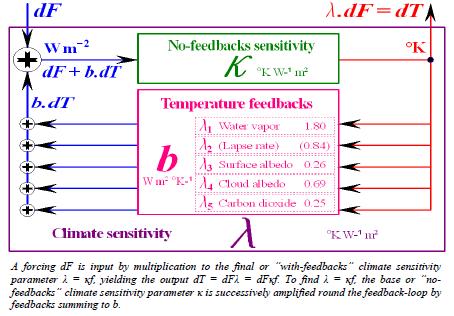
Figure 3
Bode (1945) feedback amplification schematic

For the first time, IPCC (2007) quantifies the key individual temperature feedbacks summing to b:
“In AOGCMs, the water vapor feedback constitutes by far the strongest feedback, with a multi-model mean and standard deviation … of 1.80 ± 0.18 W m–2 K–1, followed by the negative lapse rate feedback (–0.84 ± 0.26 W m–2 K–1) and the surface albedo feedback (0.26 ± 0.08 W m–2 K–1). The cloud feedback mean is 0.69 W m–2 K–1 with a very large inter-model spread of ±0.38 W m–2K–1.” (Soden & Held, 2006).
To these we add the CO2 feedback, which IPCC (2007, ch.7) separately expresses not as W m–2 °K–1 but as concentration increase per CO2 doubling: [25, 225] ppmv, central estimate q = 87 ppmv. Where p is concentration at first doubling, the proportionate increase in atmospheric CO2 concentration from the CO2 feedback is o = (p + q) / p = (556 + 87) / 556 ≈ 1.16. Then the CO2 feedback is –λCO2 = z ln(o) / dTλ ≈ 5.35 ln(1.16) / 3.2 ≈ 0.25 Wm–2 K–1. (11) The CO2 feedback is added to the previously-itemized feedbacks to complete the feedback-sum b:
b = 1.8 – 0.84 + 0.26 + 0.69 + 0.25 ≈ 2.16 Wm–2 ºK–1, (12)
so that, where κ = 0.313, the IPCC’s unstated central estimate of the value of the feedback factor f is at the lower end of the range f = 3-4 suggested in Hansen et al. (1984) –
f = (1 – bκ)–1 ≈ (1 – 2.16 x 0.313)–1 ≈ 3.077. (13)
Final climate sensitivity ΔTλ, after taking account of temperature feedbacks as well as the forcings that triggered them, is simply the product of the three factors described in Eqn. (1), each of which we have briefly described above. Thus, at CO2 doubling, –
ΔTλ = ΔF2x κ f ≈ 3.405 x 0.313 x 3.077 ≈ 3.28 °K (14)
IPCC (2007) gives dTλ on [2.0, 4.5] ºK at CO2 doubling, central estimate dTλ ≈ 3.26 °K, demonstrating that the IPCC’s method has been faithfully replicated. There is a further checksum, –
ΔTκ = ΔTλ / f = κ ΔF2x = 0.313 x 3.405 ≈ 1.1 °K, (15)
sufficiently close to the IPCC’s estimate ΔTκ ≈ 1.2 °K, based on Hansen (1984), who had estimated a range 1.2-1.3 °K based on his then estimate that the radiative forcing ΔF2xCO2 arising from a CO2 doubling would amount to 4.8 W m–2, whereas the IPCC’s current estimate is ΔF2xCO2 = 3.71 W m–2 (see Eqn. 2), requiring a commensurate reduction in ΔTκ that the IPCC has not made. A final checksum is provided by Eqn. (5), giving a value identical to that of the IPCC at Eqn (7):
κ = ΔTλ / (ΔF2x + bΔTλ)
≈ 3.28 / (3.405 + 2.16 x 3.28)
≈ 0.313 °K W–1 m2. (16)
Having outlined the IPCC’s methodology, we proceed to re-evaluate each of the three factors in dTλ. None of these three factors is directly mensurable. For this and other reasons, it is not possible to obtain climate sensitivity numerically using general-circulation models: for, as Akasofu (2008) has pointed out, climate sensitivity must be an input to any such model, not an output from it. In attempting a re-evaluation of climate sensitivity, we shall face the large uncertainties inherent in the climate object, whose complexity, non-linearity, and chaoticity present formidable initial-value and boundary-value problems. We cannot measure total radiative forcing, with or without temperature feedbacks, because radiative and non-radiative atmospheric transfer processes combined with seasonal, latitudinal, and altitudinal variabilities defeat all attempts at reliable measurement. We cannot even measure changes in TS to within a factor of two (McKitrick, 2007).
Even satellite-based efforts at assessing total energy-flux imbalance for the whole Earth-troposphere system are uncertain. Worse, not one of the individual forcings or feedbacks whose magnitude is essential to an accurate evaluation of climate sensitivity is mensurable directly, because we cannot distinguish individual forcings or feedbacks one from another in the real atmosphere, we can only guess at the interactions between them, and we cannot even measure the relative contributions of all forcings and of all feedbacks to total radiative forcing. Therefore we shall adopt two approaches:
theoretical demonstration (where possible); and empirical comparison of certain outputs from the models with observation to identify any significant inconsistencies.
Radiative forcing ΔF2x reconsidered
We take the second approach with ΔF2x. Since we cannot measure any individual forcing directly in the atmosphere, the models draw upon results of laboratory experiments in passing sunlight through chambers in which atmospheric constituents are artificially varied; such experiments are, however, of limited value when translated into the real atmosphere, where radiative transfers and non-radiative transports (convection and evaporation up, advection along, subsidence and precipitation down), as well as altitudinal and latitudinal asymmetries, greatly complicate the picture. Using these laboratory values, the models attempt to produce latitude-versus-altitude plots to display the characteristic
signature of each type of forcing. The signature or fingerprint of anthropogenic greenhouse-gas forcing, as predicted by the models on which the IPCC relies, is distinct from that of any other forcing, in that the models project that the rate of change in temperature in the tropical mid-troposphere – the region some 6-10 km above the surface – will be twice or thrice the rate of change at the surface (Figure 4):
Figure 4
Temperature fingerprints of five forcings Modeled zonal

The fingerprint of anthropogenic greenhouse-gas forcing is a distinctive “hot-spot” in the tropical midtroposphere.
Figure 4 shows altitude-vs.-latitude plots from four of the IPCC’s models:
Figure 5
Fingerprints of anthropogenic warming projected by four models

However, as Douglass et al. (2004) and Douglass et al. (2007) have demonstrated, the projected
fingerprint of anthropogenic greenhouse-gas warming in the tropical mid-troposphere is not observed
in reality. Figure 6 is a plot of observed tropospheric rates of temperature change from the Hadley
Center for Forecasting. In the tropical mid-troposphere, at approximately 300 hPa pressure, the model projected
fingerprint of anthropogenic greenhouse warming is absent from this and all other observed
records of temperature changes in the satellite and radiosonde eras:
Continue to Part 3


