Climate Sensitivity Reconsidered Part 1

A special report from Christopher Monckton of Brenchley for all Climate Alarmists, Consensus Theorists and Anthropogenic Global Warming Supporters

January 20, 2011

Abstract

The Intergovernmental Panel on Climate Change (IPCC, 2007) concluded that anthropogenic CO2 emissions probably
caused more than half of the “global warming” of the past 50 years and would cause further rapid warming. However,
global mean surface temperature TS has not risen since 1998 and may have fallen since late 2001. The present analysis
suggests that the failure of the IPCC’s models to predict this and many other climatic phenomena arises from defects in its
evaluation of the three factors whose product is climate sensitivity:

1) Radiative forcing ΔF;
2) The no-feedbacks climate sensitivity parameter κ; and
3) The feedback multiplier f.
Some reasons why the IPCC’s estimates may be excessive and unsafe are explained. More importantly, the conclusion is
that, perhaps, there is no “climate crisis”, and that currently-fashionable efforts by governments to reduce anthropogenic
CO2 emissions are pointless, may be ill-conceived, and could even be harmful.

The context

LOBALLY-AVERAGED land and sea surface absolute temperature TS has not risen since 1998 (Hadley Center; US National Climatic Data Center; University of Alabama at Huntsville; etc.). For almost seven years, TS may even have fallen (Figure 1). There may be no new peak until 2015 (Keenlyside et al., 2008).

The models heavily relied upon by the Intergovernmental Panel on Climate Change (IPCC) had not projected this multidecadal stasis in “global warming”; nor (until trained ex post facto) the fall in TS from 1940-1975; nor 50 years’ cooling in Antarctica (Doran et al., 2002) and the Arctic (Soon, 2005); nor the absence of ocean warming since 2003 (Lyman et al., 2006; Gouretski & Koltermann, 2007); nor the onset, duration, or intensity of the Madden-Julian intraseasonal oscillation, the Quasi-Biennial Oscillation in the tropical stratosphere, El Nino/La Nina oscillations, the Atlantic Multidecadal Oscillation, or the Pacific Decadal Oscillation that has recently transited from its warming to its cooling phase (oceanic oscillations which, on their own, may account for all of the observed warmings and coolings over the past half-century: Tsonis et al., 2007); nor the magnitude nor duration of multicentury events such as the Medieval Warm Period or the Little Ice Age; nor the cessation since 2000 of the previously-observed growth in atmospheric methane concentration (IPCC, 2007); nor the active 2004 hurricane season; nor the inactive subsequent seasons; nor the UK flooding of 2007 (the Met Office had forecast a summer of prolonged droughts only six weeks previously); nor the solar Grand Maximum of the past 70 years, during which the Sun was more active, for longer, than at almost any
similar period in the past 11,400 years (Hathaway, 2004; Solanki et al., 2005); nor the consequent surface “global warming” on Mars, Jupiter, Neptune’s largest moon, and even distant Pluto; nor the eerily- continuing 2006 solar minimum; nor the consequent, precipitate decline of ~0.8 °C in TS from January 2007 to May 2008 that has canceled out almost all of the observed warming of the 20th century.

Figure 1
Mean global surface temperature anomalies (°C), 2001-2008


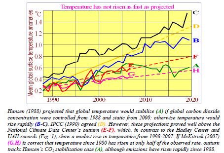
An early projection of the trend in TS in response to “global warming” was that of Hansen (1988), amplifying Hansen (1984) on quantification of climate sensitivity. In 1988, Hansen showed Congress a graph projecting rapid increases in TS to 2020 through “global warming” (Fig. 2):

Figure 2
Global temperature projections and outturns, 1988-2020


To what extent, then, has humankind warmed the world, and how much warmer will the world become if the current rate of increase in anthropogenic CO2 emissions continues? Estimating “climate sensitivity” – the magnitude of the change in TS after doubling CO2 concentration from the pre-industrial 278 parts per million to ~550 ppm – is the central question in the scientific debate about the climate. The official answer is given in IPCC (2007):

“It is very likely that anthropogenic greenhouse gas increases caused most of the observed increase in [TS] since the mid-20th century. … The equilibrium global average warming expected if carbon dioxide concentrations were to be sustained at 550 ppm is likely to be in the range 2-4.5 °C above pre-industrial values, with a best estimate of about 3 °C.”

Here as elsewhere the IPCC assigns a 90% confidence interval to “very likely”, rather than the customary 95% (two standard deviations). There is no good statistical basis for any such quantification, for the object to which it is applied is, in the formal sense, chaotic. The climate is “a complex, nonlinear, chaotic object” that defies long-run prediction of its future states (IPCC, 2001), unless the initial state of its millions of variables is known to a precision that is in practice unattainable, as Lorenz (1963; and see Giorgi, 2005) concluded in the celebrated paper that founded chaos theory –
“Prediction of the sufficiently distant future is impossible by any method, unless the present conditions are known exactly. In view of the inevitable inaccuracy and incompleteness of weather observations, precise, very-long-range weather forecasting would seem to be nonexistent.”  The Summary for Policymakers in IPCC (2007) says –“The CO2 radiative forcing increased by 20% in the last 10 years (1995-2005).”

Natural or anthropogenic CO2 in the atmosphere induces a “radiative forcing” ΔF, defined by IPCC (2001: ch.6.1) as a change in net (down minus up) radiant-energy flux at the tropopause in response to a perturbation. Aggregate forcing is natural (pre-1750) plus anthropogenic-era (post-1750) forcing. At 1990, aggregate forcing from CO2 concentration was ~27 W m–2 (Kiehl & Trenberth, 1997). From 1995-2005, CO2 concentration rose 5%, from 360 to 378 W m–2, with a consequent increase in aggregate forcing (from Eqn. 3 below) of ~0.26 W m–2, or <1%. That is one-twentieth of the value
stated by the IPCC. The absence of any definition of “radiative forcing” in the 2007 Summary led many to believe that the aggregate (as opposed to anthropogenic) effect of CO2 on TS had increased by 20% in 10 years. The IPCC – despite requests for correction – retained this confusing statement in its report.  Such solecisms throughout the IPCC’s assessment reports (including the insertion, after the scientists had completed their final draft, of a table in which four decimal points had been right-shifted so as to multiply tenfold the observed contribution of ice-sheets and glaciers to sea-level rise), combined with a heavy reliance upon computer models unskilled even in short-term projection, with initial values of key
variables unmeasurable and unknown, with advancement of multiple, untestable, non-Popperfalsifiable theories, with a quantitative assignment of unduly high statistical confidence levels to nonquantitative statements that are ineluctably subject to very large uncertainties, and, above all, with the now-prolonged failure of TS to rise as predicted (Figures 1, 2), raise questions about the reliability and hence policy-relevance of the IPCC’s central projections.

Dr. Rajendra Pachauri, chairman of the UN Intergovernmental Panel on Climate Change (IPCC), has recently said that the IPCC’s evaluation of climate sensitivity must now be revisited. This paper is a respectful contribution to that re-examination.

The IPCC’s method of evaluating climate sensitivity

We begin with an outline of the IPCC’s method of evaluating climate sensitivity. For clarity we will concentrate on central estimates. The IPCC defines climate sensitivity as equilibrium temperature change ΔTλ in response to all anthropogenic-era radiative forcings and consequent “temperature feedbacks” – further changes in TS that occur because TS has already changed in response to a forcing – arising in response to the doubling of pre-industrial CO2 concentration (expected later this century).  ΔTλ is, at its simplest, the product of three factors: the sum ΔF2x of all anthropogenic-era radiative forcings at CO2 doubling; the base or “no-feedbacks” climate sensitivity parameter κ; and the feedback
multiplier f, such that the final or “with-feedbacks” climate sensitivity parameter λ = κ f. Thus –

ΔTλ = ΔF2x κ f = ΔF2x λ, (1)
where f = (1 – bκ)–1, (2)

such that b is the sum of all climate-relevant temperature feedbacks. The definition of f in Eqn. (2) will be explained later. We now describe seriatim each of the three factors in ΔTλ: namely, ΔF2x, κ, and f.

1. Radiative forcing ΔFCO2, where (C/C0) is a proportionate increase in CO2 concentration, is given by several formulae in IPCC (2001, 2007). The simplest, following Myrhe (1998), is Eqn. (3) –

ΔFCO2 ≈ 5.35 ln(C/C0) ==> ΔF2xCO2 ≈ 5.35 ln 2 ≈ 3.708 W m–2. (3)

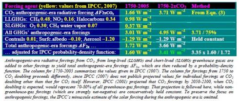
To ΔF2xCO2 is added the slightly net-negative sum of all other anthropogenic-era radiative forcings, calculated from IPCC values (Table 1), to obtain total anthropogenic-era radiative forcing ΔF2x at CO2 doubling (Eqn. 3). Note that forcings occurring in the anthropogenic era may not be anthropogenic.

Table 1
Evaluation of ΔF2x from the IPCC’s anthropogenic-era forcings


From the anthropogenic-era forcings summarized in Table 1, we obtain the first of the three factors –
ΔF2x ≈ 3.405 Wm–2. (4)

Continue to Part 2

Climate Sensitivity Reconsidered Part 2

A special report from Christopher Monckton of Brenchley to all Climate Alarmists, Consensus Theorists and Anthropogenic Global Warming Supporters

Continues from Part 1

2. The base or “no-feedbacks” climate sensitivity parameter κ, where ΔTκ is the response of TS to radiative forcings ignoring temperature feedbacks, ΔTλ is the response of TS to feedbacks as well as forcings, and b is the sum in W m–2 °K–1 of all individual temperature feedbacks, is –

κ = ΔTκ / ΔF2x °K W–1 m2, by definition; (5)
= ΔTλ / (ΔF2x + bΔTλ) °K W–1 m2. (6)

In Eqn. (5), ΔTκ, estimated by Hansen (1984) and IPCC (2007) as 1.2-1.3 °K at CO2 doubling, is the change in surface temperature in response to a tropopausal forcing ΔF2x, ignoring any feedbacks.  ΔTκ is not directly mensurable in the atmosphere because feedbacks as well as forcings are present.  Instruments cannot distinguish between them. However, from Eqn. (2) we may substitute 1 / (1 – bκ) for f in Eqn. (1), rearranging terms to yield a useful second identity, Eqn. (6), expressing κ in terms of ΔTλ, which is mensurable, albeit with difficulty and subject to great uncertainty (McKitrick, 2007).  IPCC (2007) does not mention κ and, therefore, provides neither error-bars nor a “Level of Scientific
Understanding” (the IPCC’s subjective measure of the extent to which enough is known about a variable to render it useful in quantifying climate sensitivity). However, its implicit value κ ≈ 0.313 °K W–1 m2, shown in Eqn. 7, may be derived using Eqns. 9-10 below, showing it to be the reciprocal of the estimated “uniform-temperature” radiative cooling response–

“Under these simplifying assumptions the amplification [f] of the global warming from a feedback parameter [b] (in W m–2 °C–1) with no other feedbacks operating is 1 / (1 –[bκ –1]), where [–κ –1] is the ‘uniform temperature’ radiative cooling response (of value approximately –3.2 W m–2 °C–1; Bony et al., 2006). If n independent feedbacks operate, [b] is replaced by (λ1 + λ 2+ … λ n).” (IPCC, 2007: ch.8, footnote).

Thus, κ ≈ 3.2–1 ≈ 0.313 °K W–1 m2. (7)

3. The feedback multiplier f is a unitless variable by which the base forcing is multiplied to take account of mutually-amplified temperature feedbacks. A “temperature feedback” is a change in TS that occurs precisely because TS has already changed in response to a forcing or combination of forcings.  An instance: as the atmosphere warms in response to a forcing, the carrying capacity of the space occupied by the atmosphere for water vapor increases near-exponentially in accordance with the Clausius-Clapeyron relation. Since water vapor is the most important greenhouse gas, the growth in its
concentration caused by atmospheric warming exerts an additional forcing, causing temperature to rise further. This is the “water-vapor feedback”. Some 20 temperature feedbacks have been described, though none can be directly measured. Most have little impact on temperature. The value of each feedback, the interactions between feedbacks and forcings, and the interactions between feedbacks and other feedbacks, are subject to very large uncertainties.

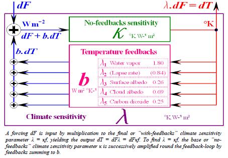
Each feedback, having been triggered by a change in atmospheric temperature, itself causes a temperature change. Consequently, temperature feedbacks amplify one another. IPCC (2007: ch.8) defines f in terms of a form of the feedback-amplification function for electronic circuits given in Bode (1945), where b is the sum of all individual feedbacks before they are mutually amplified:

f = (1 – bκ)–1 (8)
= ΔTλ / ΔTκ

Note the dependence of f not only upon the feedback-sum b but also upon κ –

ΔTλ = (ΔF + bΔTλ)κ
==> ΔTλ (1 – bκ) = ΔFκ
==> ΔTλ = ΔFκ(1 – bκ)–1
==> ΔTλ / ΔF = λ = κ(1 – bκ)–1 = κf
==> f = (1 – bκ)–1 ≈ (1 – b / 3.2)–1
==> κ ≈ 3.2–1 ≈ 0.313 °K W–1 m2. (9)

Equivalently, expressing the feedback loop as the sum of an infinite series,

ΔTλ = ΔFκ + ΔFκ 2b + ΔFκ 2b2 + …
= ΔFκ(1 + κb + κb2 + …)
= ΔFκ(1 – κb)–1
= ΔFκf
==> λ = ΔTλ /ΔF = κf (10)

Figure 3
Bode (1945) feedback amplification schematic


For the first time, IPCC (2007) quantifies the key individual temperature feedbacks summing to b:
“In AOGCMs, the water vapor feedback constitutes by far the strongest feedback, with a multi-model mean and standard deviation … of 1.80 ± 0.18 W m–2 K–1, followed by the negative lapse rate feedback (–0.84 ± 0.26 W m–2 K–1) and the surface albedo feedback (0.26 ± 0.08 W m–2 K–1). The cloud feedback mean is 0.69 W m–2 K–1 with a very large inter-model spread of ±0.38 W m–2K–1.” (Soden & Held, 2006).

To these we add the CO2 feedback, which IPCC (2007, ch.7) separately expresses not as W m–2 °K–1 but as concentration increase per CO2 doubling: [25, 225] ppmv, central estimate q = 87 ppmv. Where p is concentration at first doubling, the proportionate increase in atmospheric CO2 concentration from the CO2 feedback is o = (p + q) / p = (556 + 87) / 556 ≈ 1.16. Then the CO2 feedback is –λCO2 = z ln(o) / dTλ ≈ 5.35 ln(1.16) / 3.2 ≈ 0.25 Wm–2 K–1. (11) The CO2 feedback is added to the previously-itemized feedbacks to complete the feedback-sum b:

b = 1.8 – 0.84 + 0.26 + 0.69 + 0.25 ≈ 2.16 Wm–2 ºK–1, (12)

so that, where κ = 0.313, the IPCC’s unstated central estimate of the value of the feedback factor f is at the lower end of the range f = 3-4 suggested in Hansen et al. (1984) –

f = (1 – bκ)–1 ≈ (1 – 2.16 x 0.313)–1 ≈ 3.077. (13)

Final climate sensitivity ΔTλ, after taking account of temperature feedbacks as well as the forcings that triggered them, is simply the product of the three factors described in Eqn. (1), each of which we have briefly described above. Thus, at CO2 doubling, –

ΔTλ = ΔF2x κ f ≈ 3.405 x 0.313 x 3.077 ≈ 3.28 °K (14)

IPCC (2007) gives dTλ on [2.0, 4.5] ºK at CO2 doubling, central estimate dTλ ≈ 3.26 °K, demonstrating that the IPCC’s method has been faithfully replicated. There is a further checksum, –

ΔTκ = ΔTλ / f = κ ΔF2x = 0.313 x 3.405 ≈ 1.1 °K, (15)

sufficiently close to the IPCC’s estimate ΔTκ ≈ 1.2 °K, based on Hansen (1984), who had estimated a range 1.2-1.3 °K based on his then estimate that the radiative forcing ΔF2xCO2 arising from a CO2 doubling would amount to 4.8 W m–2, whereas the IPCC’s current estimate is ΔF2xCO2 = 3.71 W m–2 (see Eqn. 2), requiring a commensurate reduction in ΔTκ that the IPCC has not made.  A final checksum is provided by Eqn. (5), giving a value identical to that of the IPCC at Eqn (7):

κ = ΔTλ / (ΔF2x + bΔTλ)
≈ 3.28 / (3.405 + 2.16 x 3.28)
≈ 0.313 °K W–1 m2. (16)

Having outlined the IPCC’s methodology, we proceed to re-evaluate each of the three factors in dTλ.  None of these three factors is directly mensurable. For this and other reasons, it is not possible to obtain climate sensitivity numerically using general-circulation models: for, as Akasofu (2008) has pointed out, climate sensitivity must be an input to any such model, not an output from it.  In attempting a re-evaluation of climate sensitivity, we shall face the large uncertainties inherent in the climate object, whose complexity, non-linearity, and chaoticity present formidable initial-value and boundary-value problems. We cannot measure total radiative forcing, with or without temperature feedbacks, because radiative and non-radiative atmospheric transfer processes combined with seasonal, latitudinal, and altitudinal variabilities defeat all attempts at reliable measurement. We cannot even measure changes in TS to within a factor of two (McKitrick, 2007).

Even satellite-based efforts at assessing total energy-flux imbalance for the whole Earth-troposphere system are uncertain. Worse, not one of the individual forcings or feedbacks whose magnitude is essential to an accurate evaluation of climate sensitivity is mensurable directly, because we cannot distinguish individual forcings or feedbacks one from another in the real atmosphere, we can only guess at the interactions between them, and we cannot even measure the relative contributions of all forcings and of all feedbacks to total radiative forcing. Therefore we shall adopt two approaches:
theoretical demonstration (where possible); and empirical comparison of certain outputs from the models with observation to identify any significant inconsistencies.

Radiative forcing ΔF2x reconsidered

We take the second approach with ΔF2x. Since we cannot measure any individual forcing directly in the atmosphere, the models draw upon results of laboratory experiments in passing sunlight through chambers in which atmospheric constituents are artificially varied; such experiments are, however, of limited value when translated into the real atmosphere, where radiative transfers and non-radiative transports (convection and evaporation up, advection along, subsidence and precipitation down), as well as altitudinal and latitudinal asymmetries, greatly complicate the picture. Using these laboratory values, the models attempt to produce latitude-versus-altitude plots to display the characteristic
signature of each type of forcing. The signature or fingerprint of anthropogenic greenhouse-gas forcing, as predicted by the models on which the IPCC relies, is distinct from that of any other forcing, in that the models project that the rate of change in temperature in the tropical mid-troposphere – the region some 6-10 km above the surface – will be twice or thrice the rate of change at the surface (Figure 4):

Figure 4
Temperature fingerprints of five forcings Modeled zonal


The fingerprint of anthropogenic greenhouse-gas forcing is a distinctive “hot-spot” in the tropical midtroposphere.
Figure 4 shows altitude-vs.-latitude plots from four of the IPCC’s models:

Figure 5
Fingerprints of anthropogenic warming projected by four models


However, as Douglass et al. (2004) and Douglass et al. (2007) have demonstrated, the projected
fingerprint of anthropogenic greenhouse-gas warming in the tropical mid-troposphere is not observed
in reality. Figure 6 is a plot of observed tropospheric rates of temperature change from the Hadley
Center for Forecasting. In the tropical mid-troposphere, at approximately 300 hPa pressure, the model projected
fingerprint of anthropogenic greenhouse warming is absent from this and all other observed
records of temperature changes in the satellite and radiosonde eras:

Continue to Part 3

Daftar Akun Bandar Togel Resmi dengan Hadiah 4D 10 Juta Tahun 2024

Togel resmi adalah langkah penting bagi para penggemar togel yang ingin menikmati permainan dengan aman dan terpercaya. Tahun 2024 menawarkan berbagai kesempatan menarik, termasuk hadiah 4D sebesar 10 juta rupiah yang bisa Anda menangkan. Anda perlu mendaftar akun di Daftar Togel yang menawarkan hadiah tersebut. Proses pendaftaran biasanya sederhana dan melibatkan pengisian formulir dengan informasi pribadi Anda serta verifikasi data untuk memastikan keamanan transaksi. Setelah akun Anda selasai terdaftar, Anda dapat berpartisipasi dalam berbagai permainan togel berbagai fitur yang disediakan oleh situs togel terbesar.

Bermain di Link Togel memungkinkan Anda memasang taruhan dengan minimal 100 perak, sehingga semua kalangan bisa ikut serta. Meskipun taruhan rendah, Anda tetap bisa memenangkan hadiah besar dan mendapatkan bonus. Untuk mulai bermain, Anda harus mendaftar terlebih dahulu.

Bagi pemain togel yang ingin menikmati diskon terbesar, mendaftar di situs togel online terpercaya adalah langkah yang tepat. Bo Togel Hadiah 2d 200rb tidak hanya memberikan jaminan keamanan dalam bertransaksi, tetapi juga menawarkan berbagai diskon untuk jenis taruhan tertentu. Diskon yang besar ini memungkinkan pemain untuk menghemat lebih banyak dan memasang taruhan dalam jumlah yang lebih banyak. Dengan begitu, peluang untuk mendapatkan hadiah juga semakin tinggi, sekaligus memastikan bahwa setiap taruhan dilakukan di situs yang aman dan resmi.

Link Slot Gacor Terpercaya untuk Menang Setiap Hari

Slot gacor hari ini menjadi incaran para pemain Link Slot Gacor yang ingin menikmati peluang jackpot besar hanya dengan menggunakan modal kecil, sehingga mereka bisa merasakan pengalaman bermain yang lebih menyenangkan dan penuh keuntungan.

Situs dengan slot Mahjong Ways gacor memberikan jackpot dan Scatter Hitam lebih sering di tahun 2024. Pastikan memilih situs terpercaya yang menyediakan fitur scatter unggulan, sehingga peluang Anda untuk menang lebih besar dan aman.

Dengan Situs Slot Depo 5k, Anda bisa bermain dengan modal kecil namun tetap memiliki kesempatan besar untuk meraih hadiah. Banyak platform judi online kini menawarkan pilihan deposit rendah ini, sehingga pemain dengan budget terbatas tetap bisa menikmati permainan slot favorit mereka. Bermain slot dengan deposit kecil seperti ini tentu memberikan kenyamanan bagi pemain baru maupun veteran.

Situs Slot Gacor Gampang Menang RTP Live Tertinggi

Strategi bermain slot online kini semakin berkembang, terutama dengan munculnya data rtp slot gacor tertinggi. Para pemain dapat memanfaatkan rtp live untuk memilih slot gacor dengan rtp slot yang terbaik, memastikan mereka memiliki peluang menang yang lebih besar. Slot rtp tertinggi yang tersedia hari ini bisa menjadi panduan penting bagi siapa saja yang ingin menikmati permainan yang lebih menguntungkan. Dengan memahami rtp slot online, pemain dapat bermain dengan lebih strategis dan mendapatkan hasil yang lebih memuaskan.

Related Links:

Togel178

Pedetogel

Sabatoto

Togel279

Togel158

Colok178

Novaslot88

Lain-Lain

Partner Links